The term "Computer Graphics" is concerned with all aspects of producing pictures or images using a computer.
It encompasses the creation, manipulation, and representation of images and animations on computers.
The term "Computer Graphics" is concerned with all aspects of producing pictures or images using a computer.
It encompasses the creation, manipulation, and representation of images and animations on computers.
Computer graphics can be broadly classified into two types: two-dimensional (2D) and three-dimensional (3D) graphics.
2D Graphics: are digital images that are computer-based.
They include 2D geometric models, such as image compositions, pixel art, digital art, photographs, and text.
2D graphics or computer generated images are used everyday on traditional printing and drawing.
3D Graphics: are graphics that use 3D representation of geometric data.
This geometric data is then manipulated by computers via 3D computer graphics software in order to customize their display, movements, and appearance.
3D computer graphics are often referred to as 3d models. A 3d model is a mathematical representation of geometric data that is contained in a data file. 3D models, can be used for real-time 3D viewing in animations, videos, movies, training, simulations, architectural visualizations or for display as 2D rendered images (2D renders)
The development of computer graphics has been driven both by the needs of the user community and by advances in hardware and software. The applications of computer graphics are many and varied; we can, however, divide them into four major areas:
Although many applications span two or more of these areas, the development of the field was based on separate work in each.
One of the most common uses of computer graphics is to display information in a pictorial or graphical form. This includes the generation of charts, graphs, and maps, as well as the visualization of scientific data. For example, medical imaging techniques such as MRI and CT scans use computer graphics to create detailed images of the human body.
Computer graphics is widely used in design and modeling applications, such as computer-aided design (CAD) for engineering and architectural design. It allows designers to create and manipulate 3D models of objects and structures, visualize designs from different angles, and simulate how they will look and function in the real world.
Computer graphics is also used to create realistic simulations and animations for various purposes, including entertainment, training, and scientific visualization. This includes the creation of 3D animations for movies and video games, as well as simulations for training pilots, surgeons, and other professionals.
Computer graphics plays a crucial role in the design of user interfaces for software applications. It allows developers to create visually appealing and intuitive interfaces that enhance the user experience. This includes the design of icons, buttons, menus, and other graphical elements that users interact with.
A computer graphics system is a computer system; as such, it must have all the components of a general-purpose computer system. There are six major elements in our system:
These components are shown in the figure below:
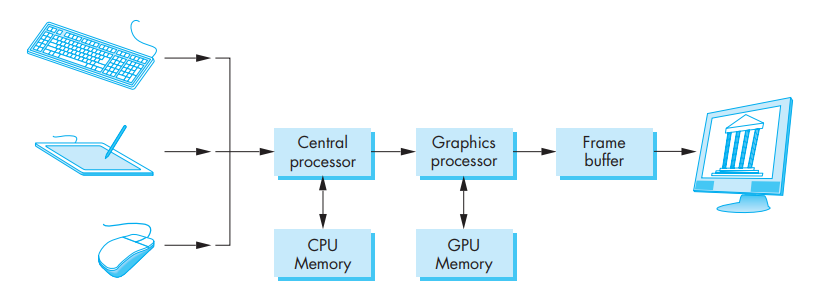
This model is general enough to include workstations and personal computers, interactive game systems, mobile phones, GPS systems, and sophisticated imagegeneration systems. Although most of the components are present in a standard computer, it is the way each element is specialized for computer graphics that characterizes this diagram as a portrait of a graphics system.
Input devices are used to capture data (and images) from the real world and convert them into a form that can be processed by the computer.
Most graphics systems provide a keyboard and at least one other input device. The most common input devices are the mouse, the joystick, and the data tablet. Each provides positional information to the system, and each usually is equipped with one or more buttons to provide signals to the processor. Often called pointing devices, these devices allow a user to indicate a particular location on the display.
Modern systems, such as game consoles, provide a much richer set of input devices, with new devices appearing almost weekly. In addition, there are devices which provide three- (and more) dimensional input. Consequently, we want to provide a flexible model for incorporating the input from such devices into our graphics programs
We can think about input devices in two distinct ways. The obvious one is to look at them as physical devices, such as a keyboard or a mouse, and to discuss how they work. Certainly, we need to know something about the physical properties of our input devices, so such a discussion is necessary if we are to obtain a full understanding of input. However, from the perspective of an application programmer, we should not need to know the details of a particular physical device to write an application program.
Rather, we prefer to treat input devices as logical devices whose properties are specified in terms of what they do from the perspective of the application program. A logical device is characterized by its high-level interface with the user program rather than by its physical characteristics.
Logical devices are familiar to all writers of highlevel programs. For example, data input and output in Java are done through classes such as System.out for output, PrintWriter for writing to files, and Scanner for input, whose methods use the standard Java data types. When we output a string using System.out.println or PrintWriter.println, the physical device on which the output appears could be a printer, a terminal, or a disk file. This output could even be the input to another program. The details of the format required by the destination device are of minor concern to the writer of the application program.
In computer graphics, the use of logical devices is slightly more complex because the forms that input can take are more varied than the strings of bits or characters to which we are usually restricted in nongraphical applications. For example, we can use the mouse—a physical device—either to select a location on the screen of our CRT or to indicate which item in a menu we wish to select. In the first case, an x, y pair (in some coordinate system) is returned to the user program; in the second, the application program may receive an integer as the identifier of an entry in the menu. The separation of physical from logical devices allows us to use the same physical devices in multiple markedly different logical ways. It also allows the same program to work, without modification, if the mouse is replaced by another physical device, such as a data tablet or trackball.
From the physical perspective, each input device has properties that make it more suitable for certain tasks than for others. We take the view used in most of the workstation literature that there are two primary types of physical devices: pointing devices and keyboard devices
The pointing device allows the user to indicate a position on the screen and almost always incorporates one or more buttons to allow the user to send signals or interrupts to the computer.
The keyboard device is almost always a physical keyboard but can be generalized to include any device that returns character codes. We use the American Standard Code for Information Interchange (ASCII) in our examples. ASCII assigns a single unsigned byte to each character. Nothing we do restricts us to this particular choice, other than that ASCII is the prevailing code used. Note, however, that other codes, especially those used for Internet applications, use multiple bytes for each character, thus allowing for a much richer set of supported characters.
The mouse and trackball are similar in use and often in construction as well. A typical mechanical mouse when turned over looks like a trackball. In both devices, the motion of the ball is converted to signals sent back to the computer by pairs of encoders inside the device that are turned by the motion of the ball. The encoders measure motion in two orthogonal directions
There are many variants of these devices. Some use optical detectors rather than mechanical detectors to measure motion. Small trackballs are popular with portable computers because they can be incorporated directly into the keyboard. There are also various pressure-sensitive devices used in keyboards that perform similar functions to the mouse and trackball but that do not move; their encoders measure the pressure exerted on a small knob that often is located between two keys in the middle of the keyboard
We can view the output of the mouse or trackball as two independent values provided by the device. These values can be considered as positions and converted— either within the graphics system or by the user program—to a two-dimensional location in a convenient coordinate system. If it is configured in this manner, we can use the device to position a marker (cursor) automatically on the display; however, we rarely use these devices in this direct manner.
It is not necessary that the output of the mouse or trackball encoders be interpreted as a position. Instead, either the device driver or a user program can interpret the information from the encoder as two independent velocities. The computer can then integrate these values to obtain a two-dimensional position.
Thus, as a mouse moves across a surface, the integrals of the velocities yield x, y values that can be converted to indicate the position for a cursor on the screen, as shown below:
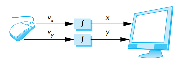
By interpreting the distance traveled by the ball as a velocity, we can use the device as a variable-sensitivity input device. Small deviations from rest cause slow or small changes; large deviations cause rapid large changes.
With either device, if the ball does not rotate, then there is no change in the integrals and a cursor tracking the position of the mouse will not move.
In this mode, these devices are relative-positioning devices because changes in the position of the ball yield a position in the user program; the absolute location of the ball (or the mouse) is not used by the application program.
Relative positioning, as provided by a mouse or trackball, is not always desirable.
In particular, these devices are not suitable for an operation such as tracing a diagram. If, while the user is attempting to follow a curve on the screen with a mouse, she lifts and moves the mouse, the absolute position on the curve being traced is lost.
Data tablets provide absolute positioning. A typical data tablet has rows and columns of wires embedded under its surface. The position of the stylus is determined through electromagnetic interactions between signals traveling through the wires and sensors in the stylus. Touch-sensitive transparent screens that can be placed over the face of a CRT have many of the same properties as the data tablet. Small, rectangular, pressure-sensitive touchpads are embedded in the keyboards of many portable computers. These touchpads can be configured as either relative- or absolute-positioning devices.
Two major characteristics describe the logical behavior of an input device: (1) the measurements that the device returns to the user program and (2) the time when the device returns those measurements.
The logical string device in Java is similar to using character input through Scanner or BufferedReader. A physical keyboard will return a string of characters to an application program; the same string might be provided from a file, or the user may see a virtual keyboard displayed on the output and use a pointing device to generate the string of characters. Logically, all three methods are examples of a string device, and application code for using such input can be the same regardless of which physical device is used.
The physical pointing device can be used in a variety of logical ways. As a locator it can provide a position to the application in either a device-independent coordinate system, such as world coordinates, as in OpenGL, or in screen coordinates, which the application can then transform to another coordinate system. A logical pick device returns the identifier of an object on the display to the application program. It is usually implemented with the same physical device as a locator but has a separate software interface to the user program.
A widget is a graphical interactive device, provided by either the window system or a toolkit. Typical widgets include menus, scrollbars, and graphical buttons. Most widgets are implemented as special types of windows. Widgets can be used to provide additional types of logical devices. For example, a menu provides one of a number of choices as may a row of graphical buttons. A logical valuator provides analog input to the user program, usually through a widget such as a slidebar, although the same logical input could be provided by a user typing numbers into a physical keyboard.
In a simple system, there may be only one processor, the central processing unit (CPU) of the system, which must do both the normal processing and the graphical processing. The main graphical function of the processor is to take specifications of graphical primitives (such as lines, circles, and polygons) generated by application programs and to assign values to the pixels in the frame buffer that best represent these entities.
For example, a triangle is specified by its three vertices, but to display its outline by the three line segments connecting the vertices, the graphics system must generate a set of pixels that appear as line segments to the viewer. The conversion of geometric entities to pixel colors and locations in the frame buffer is known as rasterization, or scan conversion.
In early graphics systems, the frame buffer was part of the standard memory that could be directly addressed by the CPU. Today, virtually all graphics systems are characterized by special-purpose graphics processing units (GPUs), custom-tailored to carry out specific graphics functions. The GPU can be either on the mother board of the system or on a graphics card. The frame buffer is accessed through the graphics processing unit and usually is on the same circuit board as the GPU.
GPUs have evolved to where they are as complex or even more complex than CPUs. They are characterized by both special-purpose modules geared toward graphical operations and a high degree of parallelism—recent GPUs contain over 100 processing units, each of which is user programmable. GPUs are so powerful that they can often be used as mini supercomputers for general purpose computing.
Until recently, the dominant type of display (or monitor) was the cathode-ray tube (CRT). A simplified picture of a CRT is shown below:
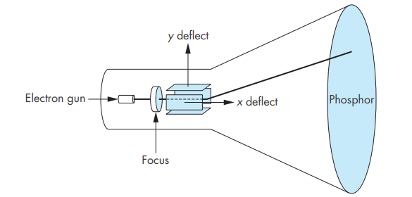
When electrons strike the phosphor coating on the tube, light is emitted. The direction of the beam is controlled by two pairs of deflection plates. The output of the computer is converted, by digitalto-analog converters, to voltages across the x and y deflection plates. Light appears on the surface of the CRT when a sufficiently intense beam of electrons is directed at the phosphor.
If the voltages steering the beam change at a constant rate, the beam will trace a straight line, visible to a viewer. Such a device is known as the random-scan, calligraphic, or vector CRT, because the beam can be moved directly from any position to any other position. If intensity of the beam is turned off, the beam can be moved to a new position without changing any visible display. This configuration was the basis of early graphics systems that predated the present raster technology
A typical CRT will emit light for only a short time—usually, a few milliseconds— after the phosphor is excited by the electron beam. For a human to see a steady, flicker-free image on most CRT displays, the same path must be retraced, or refreshed, by the beam at a sufficiently high rate, the refresh rate. In older systems, the refresh rate is determined by the frequency of the power system, 60 cycles per second or 60 Hertz (Hz) in the United States and 50 Hz in much of the rest of the world. Modern displays are no longer coupled to these low frequencies and operate at rates up to about 85 Hz.
In a raster system, the graphics system takes pixels from the frame buffer and displays them as points on the surface of the display in one of two fundamental ways.
In a noninterlaced system, the pixels are displayed row by row, or scan line by scan line, at the refresh rate.
In an interlaced display, odd rows and even rows are refreshed alternately. Interlaced displays are used in commercial television. In an interlaced display operating at 60 Hz, the screen is redrawn in its entirety only 30 times per second, although the visual system is tricked into thinking the refresh rate is 60 Hz rather than 30 Hz. Viewers located near the screen, however, can tell the difference between the interlaced and noninterlaced displays. Noninterlaced displays are becoming more widespread, even though these displays process pixels at twice the rate of the interlaced display
Color CRTs have three different colored phosphors (red, green, and blue), arranged in small groups. One common style arranges the phosphors in triangular groups called triads, each triad consisting of three phosphors, one of each primary. Most color CRTs have three electron beams, corresponding to the three types of phosphors.
In the shadow-mask CRT, a metal screen with small holes—the shadow mask—ensures that an electron beam excites only phosphors of the proper color:
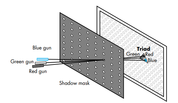
Although CRTs are still common display devices, they are rapidly being replaced by flat-screen technologies. Flat-panel monitors are inherently raster based. Although there are multiple technologies available, including light-emitting diodes (LEDs), liquid-crystal displays (LCDs), and plasma panels, all use a two-dimensional grid to address individual light-emitting elements.
The following shows a generic flat-panel monitor:
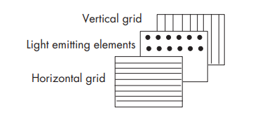
The two outside plates each contain parallel grids of wires that are oriented perpendicular to each other. By sending electrical signals to the proper wire in each grid, the electrical field at a location, determined by the intersection of two wires, can be made strong enough to control the corresponding element in the middle plate. The middle plate in an LED panel contains light-emitting diodes that can be turned on and off by the electrical signals sent to the grid. In an LCD display, the electrical field controls the polarization of the liquid crystals in the middle panel, thus turning on and off the light passing through the panel. A plasma panel uses the voltages on the grids to energize gases embedded between the glass panels holding the grids. The energized gas becomes a glowing plasma.
Most projection systems are also raster devices. These systems use a variety of technologies, including CRTs and digital light projection (DLP). From a user perspective, they act as standard monitors with similar resolutions and precisions. Hard-copy devices, such as printers and plotters, are also raster based but cannot be refreshed.
There are two kinds of 2D computer graphics: raster graphics and vector graphics.
Raster graphics, also known as bitmap graphics, are images that are made up of a grid of pixels.
The pixels are small enough that they are not easy to see individually. In fact, for many very high-resolution displays, they become essentially invisible. Each pixel in the grid has a specific color value, and together they form the complete image.
Modern screens typically use 24-bit color, where each color is defined by three 8-bit numbers representing the levels of red, green, and blue. These three primary colors combine to create any color displayed on the screen. Such systems are known as true-color, RGB-color, or full-color systems because each pixel's color is determined by the combination of red, green, and blue values.
Other formats are possible, such as grayscale, where each pixel is some shade of gray and the pixel color is given by one number that specifies the level of gray on a black-to-white scale. Typically, 256 shades of gray are used.
Early computer screens used indexed color, where only a small set of colors, usually 16 or 256, could be displayed. For an indexed color display, there is a numbered list of possible colors, and the color of a pixel is specified by an integer giving the position of the color in the list.
In any case, the color values for all the pixels on the screen are stored in a large block of memory known as a frame buffer. Changing the image on the screen requires changing color values that are stored in the frame buffer. The screen is redrawn many times per second, so that almost immediately after the color values are changed in the frame buffer, the colors of the pixels on the screen will be changed to match, and the displayed image will change.
In a very simple system, the frame buffer holds only the colored pixels that are displayed on the screen. In most systems, the frame buffer holds far more information, such as depth information needed for creating images from three-dimensional data. In these systems, the frame buffer comprises multiple buffers, one or more of which are color buffers that hold the colored pixels that are displayed. For now, we can use the terms frame buffer and color buffer synonymously without confusion.
A computer screen used in this way is the basic model of raster graphics. The term "raster" technically refers to the mechanism used on older vacuum tube computer monitors: An electron beam would move along the rows of pixels, making them glow. The beam was moved across the screen by powerful magnets that would deflect the path of the electrons. The stronger the beam, the brighter the glow of the pixel, so the brightness of the pixels could be controlled by modulating the intensity of the electron beam. The color values stored in the frame buffer were used to determine the intensity of the electron beam. (For a color screen, each pixel had a red dot, a green dot, and a blue dot, which were separately illuminated by the beam.)
Virtually all modern graphics systems are raster based. The image we see on the output device is an array—the raster—of picture elements, or pixels, produced by the graphics system.
Raster graphics are best suited for representing complex images with many colors and gradients, such as photographs and detailed illustrations.
Although images on the computer screen are represented using pixels, specifying individual pixel colors is not always the best way to create an image. Another way is to specify the basic geometric objects that it contains, shapes such as lines, circles, triangles, and rectangles. This is the idea that defines vector graphics: Represent an image as a list of the geometric shapes that it contains.
To make things more interesting, the shapes can have attributes, such as the thickness of a line or the color that fills a rectangle. Of course, not every image can be composed from simple geometric shapes. This approach certainly wouldn't work for a picture of a beautiful sunset (or for most any other photographic image). However, it works well for many types of images, such as architectural blueprints and scientific illustrations.
In fact, early in the history of computing, vector graphics was even used directly on computer screens. When the first graphical computer displays were developed, raster displays were too slow and expensive to be practical. Fortunately, it was possible to use vacuum tube technology in another way: The electron beam could be made to directly draw a line on the screen, simply by sweeping the beam along that line. A vector graphics display would store a display list of lines that should appear on the screen. Since a point on the screen would glow only very briefly after being illuminated by the electron beam, the graphics display would go through the display list over and over, continually redrawing all the lines on the list. To change the image, it would only be necessary to change the contents of the display list. Of course, if the display list became too long, the image would start to flicker because a line would have a chance to visibly fade before its next turn to be redrawn
But here is the point: For an image that can be specified as a reasonably small number of geometric shapes, the amount of information needed to represent the image is much smaller using a vector representation than using a raster representation. Consider an image made up of one thousand line segments. For a vector representation of the image, We only need to store the coordinates of two thousand points, the endpoints of the lines. This would take up only a few kilobytes of memory. To store the image in a frame buffer for a raster display would require much more memory. Similarly, a vector display could draw the lines on the screen more quickly than a raster display could copy the same image from the frame buffer to the screen. (As soon as raster displays became fast and inexpensive, however, they quickly displaced vector displays because of their ability to display all types of images reasonably well.)
Unlike raster graphics, vector graphics are resolution-independent, meaning that they can be scaled to any size without losing quality. This is because instead of pixels, vector graphics use points, lines, and curves to represent elements. This allows for scalable graphics that can be resized without loss of quality.
Vector graphics are best suited for representing simple images with solid colors and sharp edges, such as logos and icons, and widely used in graphic design, architectural design, and illustration industries.
In summary, raster graphics are made up of pixels and are best suited for complex images with many colors, while vector graphics are made up of lines and curves and are best suited for simple images with solid colors.
The divide between raster graphics and vector graphics persists in several areas of computer graphics.
For example, it can be seen in a division between two categories of programs that can be used to create images: painting programs and drawing programs
In a painting program, the image is represented as a grid of pixels, and the user creates an image by assigning colors to pixels. This might be done by using a "drawing tool" that acts like a painter's brush, or even by tools that draw geometric shapes such as lines or rectangles. But the point in a painting program is to color the individual pixels, and it is only the pixel colors that are saved. To make this clearer, suppose that We use a painting program to draw a house, then draw a tree in front of the house. If We then erase the tree, We'll only reveal a blank background, not a house. In fact, the image never really contained a "house" at all—only individually colored pixels that the viewer might perceive as making up a picture of a house
In a drawing program, the user creates an image by adding geometric shapes, and the image is represented as a list of those shapes. If We place a house shape (or collection of shapes making up a house) in the image, and We then place a tree shape on top of the house, the house is still there, since it is stored in the list of shapes that the image contains. If We delete the tree, the house will still be in the image, just as it was before We added the tree. Furthermore, We should be able to select one of the shapes in the image and move it or change its size, so drawing programs offer a rich set of editing operations that are not possible in painting programs. (The reverse, however, is also true.)
A practical program for image creation and editing might combine elements of painting and drawing, although one or the other is usually dominant.
For example, a drawing program might allow the user to include a raster-type image, treating it as one shape. A painting program might let the user create “layers,” which are separate images that can be layered one on top of another to create the final image. The layers can then be manipulated much like the shapes in a drawing program (so that We could keep both our house and our tree in separate layers, even if in the image of the house is in back of the tree).
Two well-known graphics programs are Adobe Photoshop and Adobe Illustrator. Photoshop is in the category of painting programs, while Illustrator is more of a drawing program. In the world of free software, the GNU image-processing program, Gimp, is a good alternative to Photoshop, while Inkscape is a reasonably capable free drawing program
The divide between raster and vector graphics also appears in the field of graphics file formats. There are many ways to represent an image as data stored in a file. If the original image is to be recovered from the bits stored in the file, the representation must follow some exact, known specification.
Such a specification is called a graphics file format.
Some popular graphics file formats include GIF, PNG, JPEG, WebP, and SVG. Most images used on the Web are GIF, PNG, or JPEG, but most browsers also have support for SVG images and for the newer WebP format
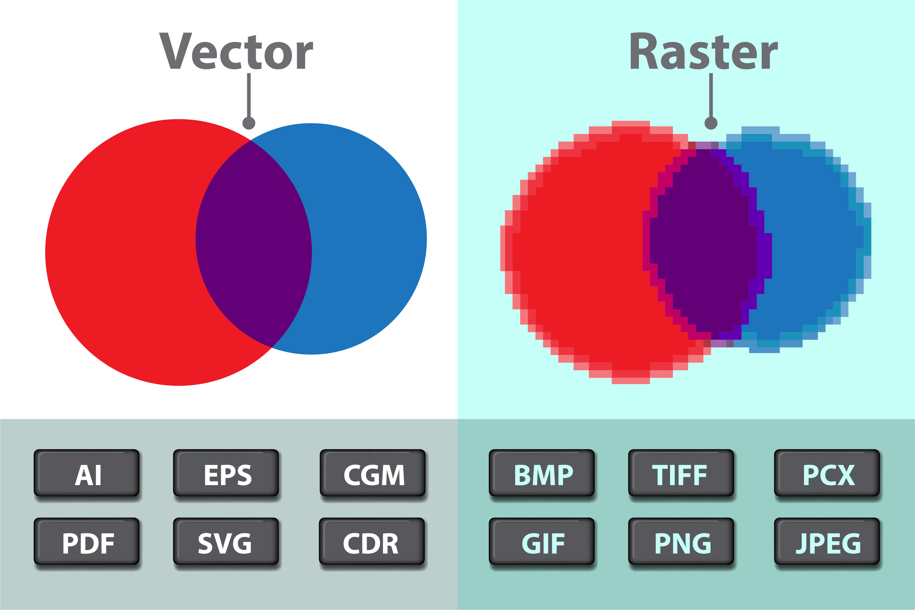
GIF, PNG, JPEG, and WebP are raster graphics formats; an image is specified by storing a color value for each pixel.
JPEG (Joint Photographic Experts Group) allows up to 16 million colors and is best for images with many colors or color gradations, especially photographs. JPEG is a "lossy" format, meaning each time the image is saved and compressed, some image information is lost, degrading quality. JPEG images allow for various levels of compression.
Low compression means high image quality, but large file size. High compression means lower image quality, but smaller file size.
GIF (Graphics Interchange Format) is a "lossless" format, meaning image quality is not degraded through compression. However, GIFs are limited to a 256-color palette, making them suitable for simpler graphics with fewer colors. GIFs also support transparent backgrounds and simple animations.
PNG (Portable Network Graphics) combines features of both JPEG and GIF. PNG supports millions of colors and transparent backgrounds. It uses lossless compression, ensuring no quality loss. However, PNGs may not be supported by older web browsers.
WebP is a modern format that supports both lossless and lossy compression, providing a balance between image quality and file size.
The amount of data necessary to represent a raster image can be quite large. However, the data usually contains a lot of redundancy and can be compressed to reduce its size. GIF and PNG use lossless compression, meaning the original image can be perfectly recovered. JPEG uses lossy compression, which allows for greater reduction in file size but at the cost of some image quality. WebP supports both types of compression.
SVG, on the other hand, is fundamentally a vector graphics format (although SVG images can include raster images). SVG is actually an XML-based language for describing twodimensional vector graphics images.
"SVG" stands for "Scalable Vector Graphics" and the term "scalable" indicates one of the advantages of vector graphics: There is no loss of quality when the size of the image is increased. A line between two points can be represented at any scale, and it is still the same perfect geometric line. If We try to greatly increase the size of a raster image, on the other hand, We will find that We don't have enough color values for all the pixels in the new image; each pixel from the original image will be expanded to cover a rectangle of pixels in the scaled image, and We will get multi-pixel blocks of uniform color. The scalable nature of SVG images make them a good choice for web browsers and for graphical elements on our computer's desktop. And indeed, some desktop environments are now using SVG images for their desktop icons.
A digital image, no matter what its format, is specified using a coordinate system. A coordinate system sets up a correspondence between numbers and geometric points. In two dimensions, each point is assigned a pair of numbers, which are called the coordinates of the point. The two coordinates of a point are often called its x -coordinate and y-coordinate, although the names "x" and "y" are arbitrary.
A raster image is a two-dimensional grid of pixels arranged into rows and columns. As such, it has a natural coordinate system in which each pixel corresponds to a pair of integers giving the number of the row and the number of the column that contain the pixel. (Even in this simple case, there is some disagreement as to whether the rows should be numbered from top-to-bottom or from bottom-to-top.)
For a vector image, it is natural to use real-number coordinates. The coordinate system for an image is arbitrary to some degree; that is, the same image can be specified using different coordinate systems.
As previously mentioned, most images viewed online are raster-based. Raster images are created with pixel-based software or captured with a camera or scanner. They are more common in general such as jpg, gif, png, and are widely used on the web.
To create these two-dimensional images, each point in the image is assigned a color.
A point in 2D can be identified by a pair of numerical coordinates. Colors can also be specified numerically.
However, the assignment of numbers to points or colors is somewhat arbitrary. So we need to spend some time studying coordinate systems, which associate numbers to points, and color models, which associate numbers to colors.
A digital image is made up of rows and columns of pixels. A pixel in such an image can be specified by saying which column and which row contains it. In terms of coordinates, a pixel can be identified by a pair of integers giving the column number and the row number.
For example, the pixel with coordinates (3,5) would lie in column number 3 and row number 5.
Conventionally, columns are numbered from left to right, starting with zero. Most graphics systems (like HTML Canvas), number rows from top to bottom starting from zero.
Some, including OpenGL, number the rows from bottom to top instead.
Note in particular that the pixel that is identified by a pair of coordinates (x,y) depends on the choice of coordinate system. We always need to know what coordinate system is in use before We know what point We are talking about.
Row and column numbers identify a pixel, not a point. A pixel contains many points; mathematically, it contains an infinite number of points. The goal of computer graphics is not really to color pixels—it is to create and manipulate images. In some ideal sense, an image should be defined by specifying a color for each point, not just for each pixel. Pixels are an approximation. If we imagine that there is a true, ideal image that we want to display, then any image that we display by coloring pixels is an approximation. This has many implications.
Suppose, for example, that we want to draw a line segment. A mathematical line has no thickness and would be invisible. So we really want to draw a thick line segment, with some specified width.
Let's say that the line should be one pixel wide.
The problem is that, unless the line is horizontal or vertical, we can't actually draw the line by coloring pixels. A diagonal geometric line will cover some pixels only partially. It is not possible to make part of a pixel black and part of it white. When We try to draw a line with black and white pixels only, the result is a jagged staircase effect.
This effect is an example of something called "aliasing".
Aliasing can also be seen in the outlines of characters drawn on the screen and in diagonal or curved boundaries between any two regions of different color. (The term aliasing likely comes from the fact that ideal images are naturally described in real-number coordinates. When We try to represent the image using pixels, many real-number coordinates will map to the same integer pixel coordinates; they can all be considered as different names or "aliases" for the same pixel.)
Anti-aliasing is a fundamental technique employed in graphics production that allows for smoother and more realistic images. This technology is used to reduce the jagged edges or "jaggies" that are commonly seen in computer-generated images, allowing them to appear as they would in real life.
It was presented by the Architecture Machine Group team, which later became known as the Media Lab, a laboratory engaged in research and development in the field of technology, science, art, design, and medicine, in 1972 at the Massachusetts Institute of Technology.
The idea is that when a pixel is only partially covered by a shape, the color of the pixel should be a mixture of the color of the shape and the color of the background. When drawing a black line on a white background, the color of a partially covered pixel would be gray, with the shade of gray depending on the fraction of the pixel that is covered by the line. (In practice, calculating this area exactly for each pixel would be too difficult, so some approximate method is used.)
At its core, anti-aliasing (also known as AA) is a method of manipulating pixels so that they appear smoother than they actually are. To achieve this effect, the software or hardware being used will sample adjacent pixels and create an average color value between them. This helps the image appear more natural and realistic since it blends together sharp pixel lines into one continuous line instead of several distinct pixelated lines.
So why does the "jagged" effect occur? Modern monitors and screens of mobile devices consist of quadrangular elements - pixels. This means that, in fact, only horizontal or vertical lines can be displayed in straight lines with clear boundaries. Angled curves are displayed as "steps". For example, the line in the picture below appears straight, but as We zoom in, it becomes clear that it is not.
Here, for example, is a geometric line, shown on the left, along with two approximations of that line made by coloring pixels. The lines are greatly magnified so that We can see the individual pixels. The line on the right is drawn using anti-aliasing, while the one in the middle is not:
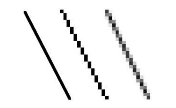
Note that anti-aliasing does not give a perfect image, but it can reduce the "jaggies" that are caused by aliasing (at least when it is viewed on a normal scale).
Anyone who has played older games is familiar with the distinctive pixelated and blocky aesthetic. "Jaggedness" occurs due to the lack of smooth transitions between colors, and anti-aliasing helps to mitigate this issue.
Jagged edges, or aliasing, occur when real-world objects with smooth, continuous curves are rasterized using pixels. This problem arises from undersampling, which happens when the sampling frequency is lower than the Nyquist Sampling Frequency, leading to a loss of information about the image.
Anti-aliasing works by sampling multiple points within and around each pixel, then calculating an average color value. This process effectively blurs the edges of objects, creating the illusion of smoother lines and reducing visible pixelation.
While anti-aliasing improves image quality, it also increases the load on the processor and graphics card, as they need to render additional shades and expend more power resources.
One way to reduce jagged edges is to increase the resolution, as higher resolution images have smaller pixels, making the blocky appearance less noticeable. However, resolution alone is not always sufficient, and software developers use various anti-aliasing techniques to further improve image quality.
There are essentially four methods of Anti-Aliasing:
Using a high-resolution display is one of the simplest methods of anti-aliasing. By increasing the resolution, more pixels can be used to represent the image, reducing the appearance of jagged edges. However, this method is limited by the physical resolution of the display and may not be practical for all applications.
Post-filtering, also known as supersampling, involves treating the screen as if it has a finer grid, effectively reducing the pixel size. The average intensity of each pixel is calculated from the intensities of subpixels, and the image is displayed at the screen resolution. This method is called post-filtering because it is done after generating the rasterized image.
Pre-filtering, or area sampling, calculates pixel intensities based on the areas of overlap between each pixel and the objects to be displayed. The final pixel color is an average of the colors of the overlapping areas. This method is called pre-filtering because it is done before generating the rasterized image.
Pixel phasing involves shifting pixel positions to approximate the positions near object geometry. Some systems allow the size of individual pixels to be adjusted to distribute intensities, which helps in pixel phasing.
Generally all anti-aliasing methods can be classified into two classifications:
Spatial anti-aliasing techniques work by sampling multiple points within each pixel and averaging the colors to reduce jagged edges.
Supersampling Anti-Aliasing (SSAA), also called full-scene anti-aliasing (FSAA), works by rendering the image at a higher resolution and then downsampling it to the display resolution. This method reduces jagged edges by averaging colors near the edges.
In this approach, a 512x512 image is first computed at higher resolution, such as 2048x2048, for example. It is then reduced through averaging or filtering to produce a 512x512 image.
While effective, SSAA is computationally intensive and can heavily load the GPU.
Multi-Sample Anti-Aliasing (MSAA) improves performance compared to SSAA by sampling multiple points within each pixel only at the edges of polygons.
Images are computed for 4 (or 8) subpixel sample points, followed by averaging. It is slow, since the frame rate is reduced by a factor of 4 (or 8). It works well for horizontal and vertical triangle edges. For other edge angles, the gaps between subpixels can cause narrow face breakups.
This method reduces the computational load while still providing good anti-aliasing quality.
Coverage Sampling Anti-Aliasing (CSAA) is an Nvidia-specific technique that improves upon MSAA by increasing the number of coverage samples without significantly increasing the number of color/depth samples. This method provides better edge quality with less performance impact.
Post-processing anti-aliasing techniques are applied after the image has been rendered to smooth out jagged edges.
Fast Approximate Anti-Aliasing (FXAA) is a post-processing technique, created by Timothy Lottes at Nvidia, that smooths edges by analyzing the final image and blending colors at the edges.
This is the cheapest and simplest smoothing algorithm.
In layman's terms, FXAA is applied to our final rendered image and works based on pixel data, not geometry. GPU's are particularly fast at executing these shader algorithms in parallel, thus it's very quick to render.
FXAA is less computationally intensive than SSAA and MSAA, making it suitable for real-time applications like video games.
Enhanced Subpixel Morphological Anti-Aliasing (SMAA) is a logical development of the FXAA algorithm. This post effect is used in post-processing the final image that combines edge detection and blending to reduce aliasing. SMAA provides high-quality anti-aliasing with a lower performance cost compared to SSAA and MSAA.
Temporal anti-aliasing techniques use information from previous frames to reduce aliasing in the current frame.
Temporal Anti-Aliasing (TAA) reduces aliasing by using information from previous frames to smooth edges in the current frame. TAA is effective at reducing flickering and shimmering in moving images, but it can introduce ghosting artifacts (visual distortions that appear in images due to a variety of factors, including movement, refraction, and sampling errors) if not implemented correctly.
There are other issues involved in mapping real-number coordinates to pixels.
For example, which point in a pixel should correspond to integer-valued coordinates such as (3,5)? The center of the pixel? One of the corners of the pixel? In general, we think of the numbers as referring to the top-left corner of the pixel.
Another way of thinking about this is to say that integer coordinates refer to the lines between pixels, rather than to the pixels themselves. But that still doesn't determine exactly which pixels are affected when a geometric shape is drawn.
For example, here are two lines drawn using HTML canvas graphics, shown greatly magnified. The lines were specified to be colored black with a one-pixel line width:

The top line was drawn from the point (100,100) to the point (120,100).
In canvas graphics, integer coordinates correspond to the lines between pixels, but when a one-pixel line is drawn, it extends one-half pixel on either side of the infinitely thin geometric line.
So for the top line, the line as it is drawn lies half in one row of pixels and half in another row. The graphics system, which uses anti-aliasing, rendered the line by coloring both rows of pixels gray.
The bottom line was drawn from the point (100.5,100.5) to (120.5,100.5). In this case, the line lies exactly along one line of pixels, which gets colored black. The gray pixels at the ends of the bottom line have to do with the fact that the line only extends halfway into the pixels at its endpoints. Other graphics systems might render the same lines differently
All this is complicated further by the fact that pixels aren't what they used to be. Pixels today are smaller!
The resolution of a display device can be measured in terms of the number of pixels per inch on the display, a quantity referred to as PPI (pixels per inch) or sometimes DPI (dots per inch).
While PPI (Pixels Per Inch) and DPI (Dots Per Inch) are often used interchangeably, they refer to different concepts and are used in different contexts.
PPI is a measure of the pixel density of a digital display, such as a computer monitor, smartphone screen, or television. It indicates the number of pixels present in one inch of the display. Higher PPI values mean more pixels are packed into each inch, resulting in sharper and more detailed images.
For example, a display with a resolution of 1920x1080 pixels and a diagonal size of 15.6 inches has a PPI of approximately 141. This means there are 141 pixels in each inch of the display.
DPI is a measure of the resolution of a printed image, indicating the number of individual dots of ink or toner that a printer can produce within one inch. Higher DPI values result in finer detail and smoother gradients in printed images.
For example, a printer with a resolution of 300 DPI can produce 300 dots of ink per inch, resulting in high-quality prints suitable for photographs and detailed graphics.
Both measures are important for ensuring high-quality visuals, but they apply to different mediums.
Early screens tended to have resolutions of somewhere close to 72 PPI. At that resolution, and at a typical viewing distance, individual pixels are clearly visible. For a while, it seemed like most displays had about 100 pixels per inch, but high resolution displays today can have 200, 300 or even 400 pixels per inch. At the highest resolutions, individual pixels can no longer be distinguished.
The fact that pixels come in such a range of sizes is a problem if we use coordinate systems based on pixels. An image created assuming that there are 100 pixels per inch will look tiny on a 400 PPI display. A one-pixel-wide line looks good at 100 PPI, but at 400 PPI, a one-pixel-wide line is probably too thin
In fact, in many graphics systems, "pixel" doesn't really refer to the size of a physical pixel. Instead, it is just another unit of measure, which is set by the system to be something appropriate. (On a desktop system, a pixel is usually about one one-hundredth of an inch. On a smart phone, which is usually viewed from a closer distance, the value might be closer to 1/160 inch. Furthermore, the meaning of a pixel as a unit of measure can change when, for example, the user applies a magnification to a web page.)
Pixels cause problems that have not been completely solved. Fortunately, they are less of a problem for vector graphics.
For vector graphics, pixels only become an issue during rasterization, the step in which a vector image is converted into pixels for display. The vector image itself can be created using any convenient coordinate system. It represents an idealized, resolution-independent image.
A rasterized image is an approximation of that ideal image, but how to do the approximation can be left to the display hardware.
When doing 2D graphics, We are given a rectangle in which We want to draw some graphics primitives. Primitives are specified using some coordinate system on the rectangle. It should be possible to select a coordinate system that is appropriate for the application. For example, if the rectangle represents a floor plan for a 15 foot by 12 foot room, then We might want to use a coordinate system in which the unit of measure is one foot and the coordinates range from 0 to 15 in the horizontal direction and 0 to 12 in the vertical direction. The unit of measure in this case is feet rather than pixels, and one foot can correspond to many pixels in the image. The coordinates for a pixel will, in general, be real numbers rather than integers. In fact, it's better to forget about pixels and just think about points in the image. A point will have a pair of coordinates given by real numbers.
To specify the coordinate system on a rectangle, We just have to specify the horizontal coordinates for the left and right edges of the rectangle and the vertical coordinates for the top and bottom. Let's call these values left, right, top, and bottom. Often, they are thought of as xmin, xmax, ymin, and ymax, but there is no reason to assume that, for example, top is less than bottom. We might want a coordinate system in which the vertical coordinate increases from bottom to top instead of from top to bottom. In that case, top will correspond to the maximum y-value instead of the minimum value.
To allow programmers to specify the coordinate system that they would like to use, it would be good to have a subroutine such as:
setCoordinateSystem(left,right,bottom,top)
The graphics system would then be responsible for automatically transforming the coordinates from the specified coordinate system into pixel coordinates. Such a subroutine might not be available, so it's useful to see how the transformation is done by hand. Let's consider the general case. Given coordinates for a point in one coordinate system, we want to find the coordinates for the same point in a second coordinate system. (Remember that a coordinate system is just a way of assigning numbers to points. It's the points that are real!)
Suppose that the horizontal and vertical limits are oldLeft, oldRight, oldTop, and oldBottom for the first coordinate system, and are newLeft, newRight, newTop, and newBottom for the second. Suppose that a point has coordinates (oldX,oldY ) in the first coordinate system. We want to find the coordinates (newX,newY ) of the point in the second coordinate system

Formulas for newX and newY are then given by:
newX = newLeft + ((oldX - oldLeft) / (oldRight - oldLeft)) * (newRight - newLeft)
newY = newTop + ((oldY - oldTop) / (oldBottom - oldTop)) * (newBottom - newTop)
The logic here is that oldX is located at a certain fraction of the distance from oldLeft to oldRight. That fraction is given by:
(oldX - oldLeft) / (oldRight - oldLeft)
The formula for newX just says that newX should lie at the same fraction of the distance from newLeft to newRight. We can also check the formulas by testing that they work when oldX is equal to oldLeft or to oldRight, and when oldY is equal to oldBottom or to oldTop.
As an example, suppose that we want to transform some real-number coordinate system with limits left, right, top, and bottom into pixel coordinates that range from 0 at left to 800 at the right and from 0 at the top 600 at the bottom. In that case, newLeft and newTop are zero, and the formulas become simply:
newX = ((oldX - left) / (right - left)) * 800
newY = ((oldY - top) / (bottom - top)) * 600
Of course, this gives newX and newY as real numbers, and they will have to be rounded or truncated to integer values if we need integer coordinates for pixels. The reverse transformation—going from pixel coordinates to real number coordinates—is also useful.
For example, if the image is displayed on a computer screen, and We want to react to mouse clicks on the image, We will probably get the mouse coordinates in terms of integer pixel coordinates, but We will want to transform those pixel coordinates into our own chosen coordinate system.
In practice, though, We won't usually have to do the transformations Werself, since most graphics APIs provide some higher level way to specify transforms.
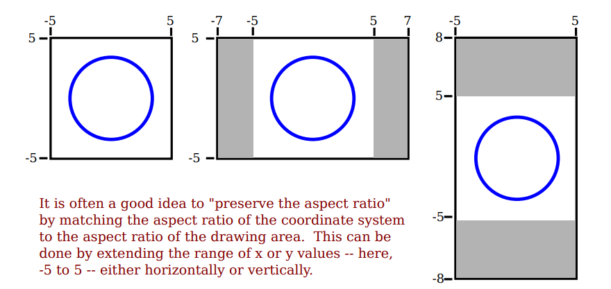
The aspect ratio of a rectangle is the ratio of its width to its height. For example an aspect ratio of 2:1 means that a rectangle is twice as wide as it is tall, and an aspect ratio of 4:3 means that the width is 4/3 times the height. Although aspect ratios are often written in the form width:height, I will use the term to refer to the fraction width/height. A square has aspect ratio equal to 1. A rectangle with aspect ratio 5/4 and height 600 has a width equal to 600*(5/4), or 750.
A coordinate system also has an aspect ratio. If the horizontal and vertical limits for the coordinate system are left, right, bottom, and top, as above, then the aspect ratio is the absolute value of:
(right - left) / (top - bottom)
If the coordinate system is used on a rectangle with the same aspect ratio, then when viewed in that rectangle, one unit in the horizontal direction will have the same apparent length as a unit in the vertical direction. If the aspect ratios don't match, then there will be some distortion.
For example, the shape defined by the equation x^2 + y^2 = 9 should be a circle, but that will only be true if the aspect ratio of the (x,y) coordinate system matches the aspect ratio of the drawing area.
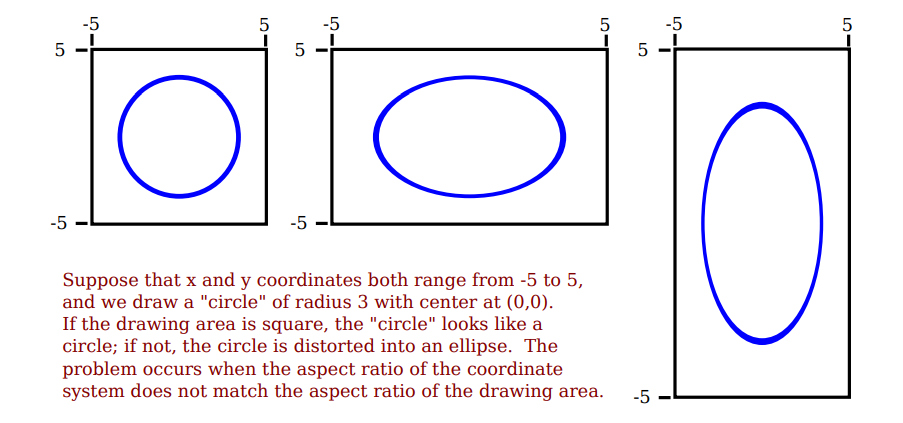
It is not always a bad thing to use different units of length in the vertical and horizontal directions. However, suppose that We want to use coordinates with limits left, right, bottom, and top, and that We do want to preserve the aspect ratio.
In that case, depending on the shape of the display rectangle, We might have to adjust the values either of left and right or of bottom and top to make the aspect ratios match:
We are talking about the most basic foundations of computer graphics. One of those is coordinate systems. The other is color.
Red, Yellow, and Blue — Primary colors. Or at least, that's what we have been told since kindergarten, isn't it? But there is more to it.
The colors on a computer screen are produced as combinations of red, green, and blue light.
Now the question is — if RYB is the primary color set then why do computers use RGB instead?
Going deep into the line, we first need to understand the color theory.
There are two different theories:
Different colors are produced by varying the intensity of each type of light. A color can be specified by three numbers giving the intensity of red, green, and blue in the color. Intensity can be specified as a number in the range zero, for minimum intensity, to one, for maximum intensity.
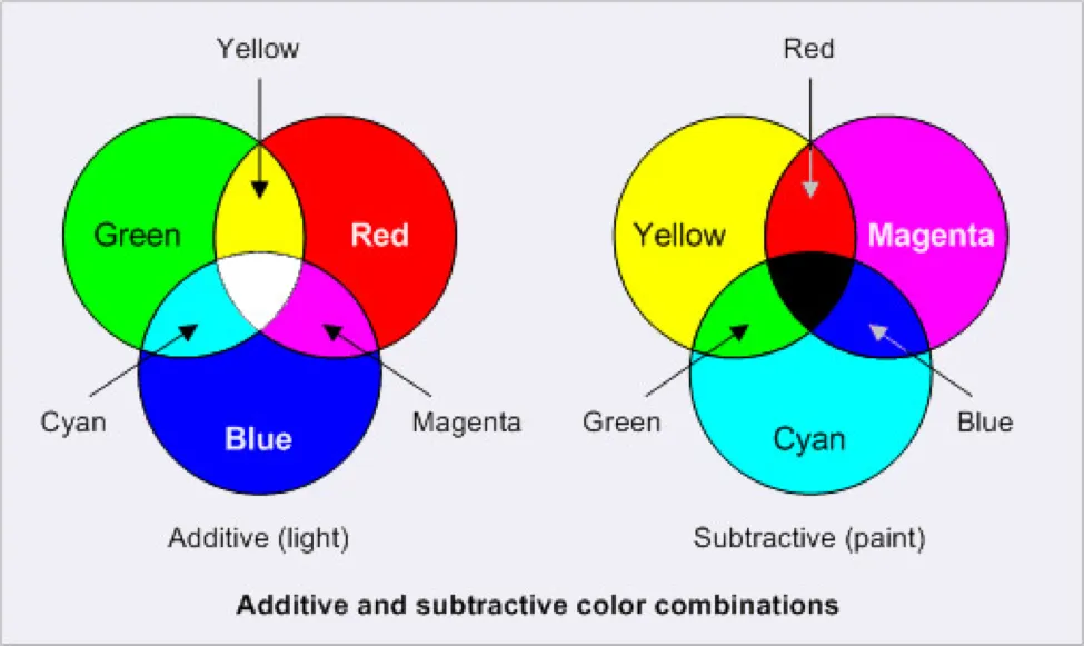
The additive is the case of the projection of one or more colored lights (wavelengths). These are the colors when mixed produce more light.
This method of specifying color is called the RGB color model, where RGB stands for Red/Green/Blue.
The red, green, and blue values for a color are called the color components of that color in the RGB color model and when mixed produces lighter colors, resulting in white light at the end. That's how our computer, TV, and other light-emitting screen works.
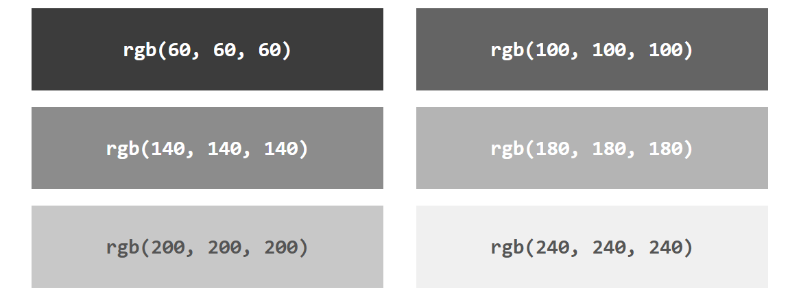
Each parameter (red, green, and blue) defines the intensity of the color with a value between 0 and 255.
This means that there are 256 x 256 x 256 = 16777216 possible colors!
For example, rgb(255, 0, 0) is displayed as red, because red is set to its highest value (255), and the other two (green and blue) are set to 0.
Another example, rgb(0, 255, 0) is displayed as green, because green is set to its highest value (255), and the other two (red and blue) are set to 0.
To display black, set all color parameters to 0, like this: rgb(0, 0, 0).
To display white, set all color parameters to 255, like this: rgb(255, 255, 255).
Shades of gray are often defined using equal values for all three parameters:
Light is made up of waves with a variety of wavelengths. A pure color is one for which all the light has the same wavelength, but in general, a color can contain many wavelengths— mathematically, an infinite number. How then can we represent all colors by combining just red, green, and blue light? In fact, we can't quite do that.
We might have heard that combinations of the three basic, or "primary" colors are sufficient to represent all colors, because the human eye has three kinds of color sensors that detect red, green, and blue light. However, that is only an approximation. The eye does contain three kinds of color sensors. The sensors are called "cone cells."
However, cone cells do not respond exclusively to red, green, and blue light. Each kind of cone cell responds, to a varying degree, to wavelengths of light in a wide range. A given mix of wavelengths will stimulate each type of cell to a certain degree, and the intensity of stimulation determines the color that we see. A different mixture of wavelengths that stimulates each type of cone cell to the same extent will be perceived as the same color.
So a perceived color can, in fact, be specified by three numbers giving the intensity of stimulation of the three types of cone cell. However, it is not possible to produce all possible patterns of stimulation by combining just three basic colors, no matter how those colors are chosen. This is just a fact about the way our eyes actually work; it might have been different.
Three basic colors can produce a reasonably large fraction of the set of perceivable colors, but there are colors that We can see in the world that We will never see on our computer screen. (This whole discussion only applies to people who actually have three kinds of cone cell. Color blindness, where someone is missing one or more kinds of cone cell, is surprisingly common.)
The range of colors that can be produced by a device such as a computer screen is called the color gamut of that device. Different computer screens can have different color gamuts, and the same RGB values can produce somewhat different colors on different screens. The color gamut of a color printer is noticeably different—and probably smaller—than the color gamut of a screen, which explains why a printed image probably doesn't look exactly the same as it did on the screen.
When we mix paints or inks, subtractive mixing results. Paints or inks are non-emissive objects here. They reflect when light falls on them. Molecules of paint absorb some of the wavelengths of light and reflect rest. That's how we see such objects.
Printers, by the way, make colors differently from the way a screen does it. Whereas a screen combines light to make a color, a printer combines inks or dyes. Because of this difference, colors meant for printers are often expressed using a different set of basic colors.
The primary colors of the subtractive mix are CMYK — Cyan, Magenta, Yellow, and K which stands for black ( To distinguish it from B for Blue. Just a convention.)
When the CMY (not K) gets mixed, it produces brownish color — a bit muddy. To get the more blackish color, the additional K for black is used. CMYK — the model used by printers & publishing houses.
In any case, the most common color model for computer graphics is RGB. RGB colors are most often represented using 8 bits per color component, a total of 24 bits to represent a color. This representation is sometimes called "24-bit color."" An 8-bit number can represent 28, or 256, different values, which we can take to be the positive integers from 0 to 255. A color is then specified as a triple of integers (r,g,b) in that range.
This representation works well because 256 shades of red, green, and blue are about as many as the eye can distinguish. In applications where images are processed by computing with color components, it is common to use additional bits per color component to avoid visual effects that might occur due to rounding errors in the computations. Such applications might use a 16-bit integer or even a 32-bit floating point value for each color component. On the other hand, sometimes fewer bits are used.
For example, one common color scheme uses 5 bits for the red and blue components and 6 bits for the green component, for a total of 16 bits for a color. (Green gets an extra bit because the eye is more sensitive to green light than to red or blue.) This “16-bit color” saves memory compared to 24-bit color and was more common when memory was more expensive.
There are many other color models besides RGB. RGB is sometimes criticized as being unintuitive. For example, it's not obvious to most people that yellow is made of a combination of red and green.
The closely related color models HSV and HSL describe the same set of colors as RGB, but attempt to do it in a more intuitive way. (HSV is sometimes called HSB, with the "B" standing for "brightness" HSV and HSB are exactly the same model.)
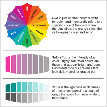
The "H" in these models stands for "hue", a basic spectral color. As H increases, the color changes from red to yellow to green to cyan to blue to magenta, and then back to red. The value of H is often taken to range from 0 to 360, since the colors can be thought of as arranged around a circle with red at both 0 and 360 degrees.
The "S" in HSV and HSL stands for "saturation" and is taken to range from 0 to 1. A saturation of 0 gives a shade of gray (the shade depending on the value of V or L). A saturation of 1 gives a "pure color" and decreasing the saturation is like adding more gray to the color.
"V" stands for "value" and "L" stands for "lightness". They determine how bright or dark the color is. The main difference is that in the HSV model, the pure spectral colors occur for V=1, while in HSL, they occur for L=0.5.
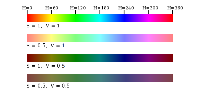
Let's look at some colors in the HSV color model. The illustration below shows colors with a full range of H-values, for S and V equal to 1 and to 0.5. Note that for S=V=1, We get bright, pure colors. S=0.5 gives paler, less saturated colors. V=0.5 gives darker colors.
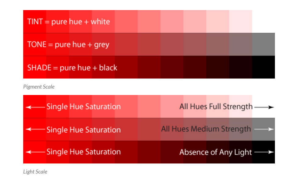
In the simple scale diagrams below, the first model indicates amount of black, white, or grey pigment added to the hue. The second model illustrates the same scale but explains the phenomenon based on light [spectral] properties.
Regardless of the two Additive and Subtractive color models, all color is a result of how our eyes physically process light waves. So let's start with the light Additive model to see how it filters into the Subtractive model and to see how hues, values and saturation interact to produce unique colors.
The three primary hues in light are red, green, and blue. Thus, that is why televisions, computer monitors, and other full-range, electronic color visual displays use a triad of red, green, and blue phosphors to produce all electronically communicated color.
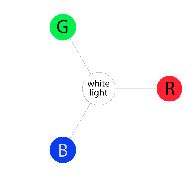
As we mentioned before, in light, all three of these wavelengths added together at full strength produces pure white light. The absence of all three of these colors produces complete darkness, or black.
Although additive and subtractive color models are considered their own unique entities for screen vs. print purposes, the hues CMY do not exist in a vacuum.
They are produced as secondary colors when RGB light hues are mixed, as follows:
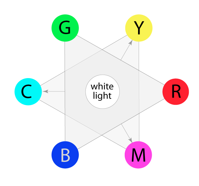
The colors on the outermost perimeter of the color circle are the "hues", which are colors in their purest form. This process can continue filling in colors around the wheel. The next level colors, the tertiary colors, are those colors between the secondary and primary colors.
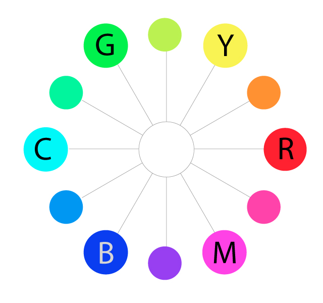
Saturation is also referred to as "intensity" and "chroma". It refers to the dominance of hue in the color. On the outer edge of the hue wheel are the 'pure' hues. As We move into the center of the wheel, the hue we are using to describe the color dominates less and less. When We reach the center of the wheel, no hue dominates. These colors directly on the central axis are considered desaturated.
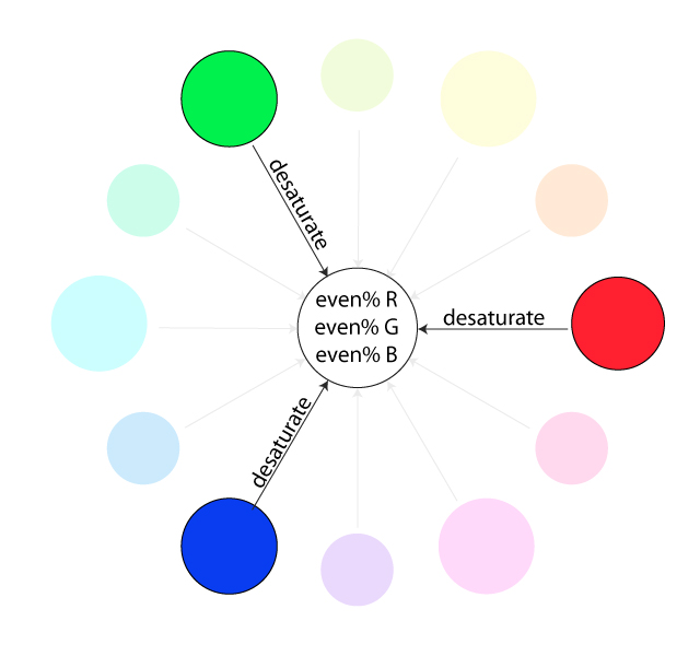
Naturally, the opposite of the image above is to saturate color.
The first example below describes the general direction color must move on the color circle to become more saturated (towards the outside). The second example depicts how a single color looks completely saturated, having no other hues present in the color.

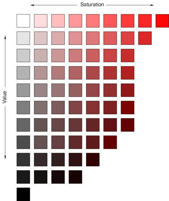
Now let's add "value" to the HSV scale. Value is the dimension of lightness/darkness. In terms of a spectral definition of color, value describes the overall intensity or strength of the light. If hue can be thought of as a dimension going around a wheel, then value is a linear axis running through the middle of the wheel, as seen below:
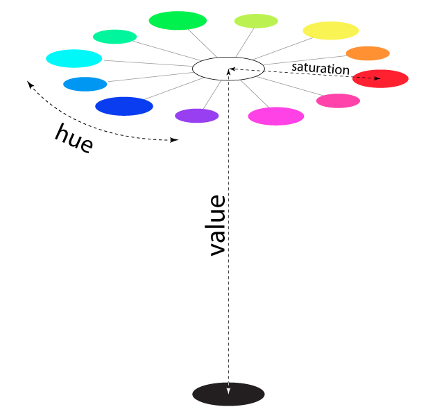
To better visualize even more, look at the example below showing a full color range for a single hue:
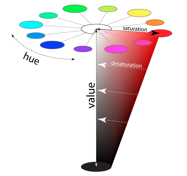
Now, if We imagine that each hue was also represented as a slice like the one above, we would have a solid, upside-down cone of colors. The example above can be considered a slice of the cone. Notice how the right-most edge of this cone slice shows the greatest amount of the dominant red hue (least amount of other competing hues), and how as We go down vertically, it gets darker in "value".
Also notice that as we travel from right to left in the cone, the hue becomes less dominant and eventually becomes completely desaturated along the vertical center of the cone. This vertical center axis of complete desaturation is referred to as grayscale.
See how this slice below translates into some isolated color swatches:
Often, a fourth component is added to color models. The fourth component is called alpha, and color models that use it are referred to by names such as RGBA and HSLA. Alpha is not a color as such. It is usually used to represent transparency.
A color with maximal alpha value is fully opaque; that is, it is not at all transparent. A color with alpha equal to zero is completely transparent and therefore invisible. Intermediate values give translucent, or partly transparent, colors.
Transparency determines what happens when We draw with one color (the foreground color) on top of another color (the background color). If the foreground color is fully opaque, it simply replaces the background color. If the foreground color is partly transparent, then it is blended with the background color.
Assuming that the alpha component ranges from 0 to 1, the color that We get can be computed as:
new_color = (alpha)*(foreground_color) + (1 - alpha)*(background_color)
This computation is done separately for the red, blue, and green color components. This is called alpha blending. The effect is like viewing the background through colored glass; the color of the glass adds a tint to the background color. This type of blending is not the only possible use of the alpha component, but it is the most common.
An RGBA color model with 8 bits per component uses a total of 32 bits to represent a color. This is a convenient number because integer values are often represented using 32-bit values. A 32-bit integer value can be interpreted as a 32-bit RGBA color.
How the color components are arranged within a 32-bit integer is somewhat arbitrary.
The most common layout is to store the alpha component in the eight high-order bits, followed by red, green, and blue. (This should probably be called ARGB color.) However, other layouts are also in use.
We have been talking about low-level graphics concepts like pixels and coordinates, but fortunately we don't usually have to work on the lowest levels. Most graphics systems let us work with higher-level shapes, such as triangles and circles, rather than individual pixels.
In a graphics API, there will be certain basic shapes that can be drawn with one command, whereas more complex shapes will require multiple commands. Exactly what qualifies as a basic shape varies from one API to another.
For example, the HTML5 canvas API provides commands to draw rectangles, circles, and lines, but not triangles. To draw a triangle, We have to draw three lines.
By "line", we really mean line segment, that is a straight line segment connecting two given points in the plane. A simple one-pixel-wide line segment, without anti-aliasing, is the most basic shape. It can be drawn by coloring pixels that lie along the infinitely thin geometric line segment.
An algorithm for drawing the line has to decide exactly which pixels to color. One of the first computer graphics algorithms, Bresenham's algorithm for line drawing, implements a very efficient procedure for doing so.
In any case, lines are typically more complicated. Anti-aliasing is one complication. Line width is another. A wide line might actually be drawn as a rectangle.
Lines can have other attributes, or properties, that affect their appearance. One question is, what should happen at the end of a wide line?
Appearance might be improved by adding a rounded "cap" on the ends of the line. A square cap—that is, extending the line by half of the line width—might also make sense.
Another question is, when two lines meet as part of a larger shape, how should the lines be joined? And many graphics systems support lines that are patterns of dashes and dots.
This illustration shows some of the possibilities:
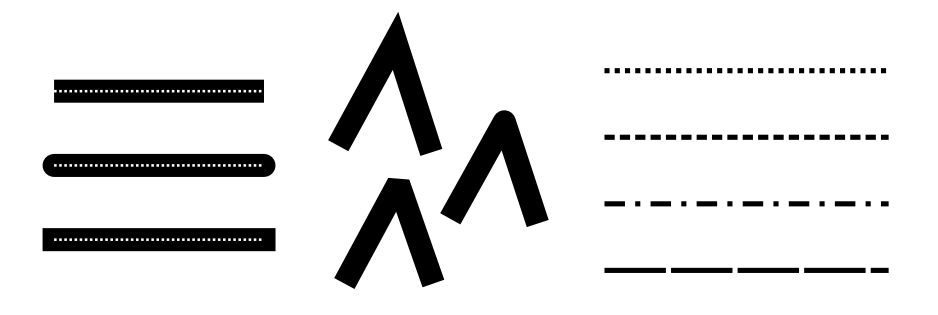
On the left are three wide lines with no cap, a round cap, and a square cap. The geometric line segment is shown as a dotted line. (The no-cap style is called “butt.”) To the right are four lines with different patterns of dots and dashes. In the middle are three different styles of line joins: mitered, rounded, and beveled.
The basic rectangular shape has sides that are vertical and horizontal. (A tilted rectangle generally has to be made by applying a rotation.) Such a rectangle can be specified with two points, (x1,y1) and (x2,y2), that give the endpoints of one of the diagonals of the rectangle. Alternatively, the width and the height can be given, along with a single base point, (x,y). In that case, the width and height have to be positive, or the rectangle is empty. The base point (x,y) will be the upper left corner of the rectangle if y increases from top to bottom, and it will be the lower left corner of the rectangle if y increases from bottom to top.

Suppose that We are given points (x1,y1) and (x2,y2), and that We want to draw the rectangle that they determine. And suppose that the only rectangle-drawing command that We have available is one that requires a point (x,y), a width, and a height. For that command, x must be the smaller of x1 and x2, and the width can be computed as the absolute value of x1 minus x2. And similarly for y and the height.
In pseudocode,

A common variation on rectangles is to allow rounded corners. For a “round rect,” the corners are replaced by elliptical arcs. The degree of rounding can be specified by giving the horizontal radius and vertical radius of the ellipse.
Here are some examples of round rects. For the shape at the right, the two radii of the ellipse are shown:

Our final basic shape is the oval. (An oval is also called an ellipse.) An oval is a closed curve that has two radii. For a basic oval, we assume that the radii are vertical and horizontal. An oval with this property can be specified by giving the rectangle that just contains it. Or it can be specified by giving its center point and the lengths of its vertical radius and its horizontal radius.
In this illustration, the oval on the left is shown with its containing rectangle and with its center point and radii:
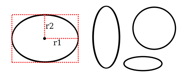
The oval on the right is a circle. A circle is just an oval in which the two radii have the same length.
If ovals are not available as basic shapes, they can be approximated by drawing a large number of line segments. The number of lines that is needed for a good approximation depends on the size of the oval. It's useful to know how to do this. Suppose that an oval has center point (x,y), horizontal radius r1, and vertical radius r2. Mathematically, the points on the oval are given by:
where angle takes on values from 0 to 360 if angles are measured in degrees or from 0 to 2π if they are measured in radians. Here sin and cos are the standard sine and cosine functions. To get an approximation for an oval, we can use this formula to generate some number of points and then connect those points with line segments.
In pseudocode, assuming that angles are measured in radians and that pi represents the mathematical constant π,

For a circle, of course, We would just have r1 = r2. This is the first time we have used the sine and cosine functions, but it won't be the last. These functions play an important role in computer graphics because of their association with circles, circular motion, and rotation. We will meet them again when we talk about transforms later.
There are two ways to make a shape visible in a drawing.
We can stroke it. Or, if it is a closed shape such as a rectangle or an oval, We can fill it.
Stroking a line is like dragging a pen along the line. Stroking a rectangle or oval is like dragging a pen along its boundary.
Filling a shape means coloring all the points that are contained inside that shape.
It's possible to both stroke and fill the same shape; in that case, the interior of the shape and the outline of the shape can have a different appearance.
When a shape intersects itself, like the two shapes in the illustration below, it's not entirely clear what should count as the interior of the shape. In fact, there are at least two different rules for filling such a shape.
In fact, there are at least two different rules for filling such a shape. Both are based on something called the winding number. The winding number of a shape about a point is, roughly, how many times the shape winds around the point in the positive direction, which we'll take here to be counterclockwise.
Winding number can be negative when the winding is in the opposite direction.
In the illustration, the shapes on the left are traced in the direction shown, and the winding number about each region is shown as a number inside the region.
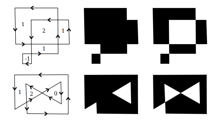
The shapes are also shown filled using the two fill rules.
For the shapes in the center, the fill rule is to color any region that has a non-zero winding number.
For the shapes shown on the right, the rule is to color any region whose winding number is odd; regions with even winding number are not filled.
There is still the question of what a shape should be filled with. Of course, it can be filled with a color, but other types of fill are possible, including patterns and gradients.
A pattern is an image, usually a small image. When used to fill a shape, a pattern can be repeated horizontally and vertically as necessary to cover the entire shape.
A gradient is similar in that it is a way for color to vary from point to point, but instead of taking the colors from an image, they are computed. There are a lot of variations to the basic idea, but there is always a line segment along which the color varies. The color is specified at the endpoints of the line segment, and possibly at additional points; between those points, the color is interpolated. The color can also be extrapolated to other points on the line that contains the line segment but lying outside the line segment; this can be done either by repeating the pattern from the line segment or by simply extending the color from the nearest endpoint.
For a linear gradient, the color is constant along lines perpendicular to the basic line segment, so we get lines of solid color going in that direction.
In a radial gradient, the color is constant along circles centered at one of the endpoints of the line segment.
And that doesn't exhaust the possibilities. To give we an idea what patterns and gradients can look like, here is a shape, filled with two gradients and two patterns:

The first shape is filled with a simple linear gradient defined by just two colors, while the second shape uses a radial gradient.
Patterns and gradients are not necessarily restricted to filling shapes. Stroking a shape is, after all, the same as filling a band of pixels along the boundary of the shape, and that can be done with a gradient or a pattern, instead of with a solid color.
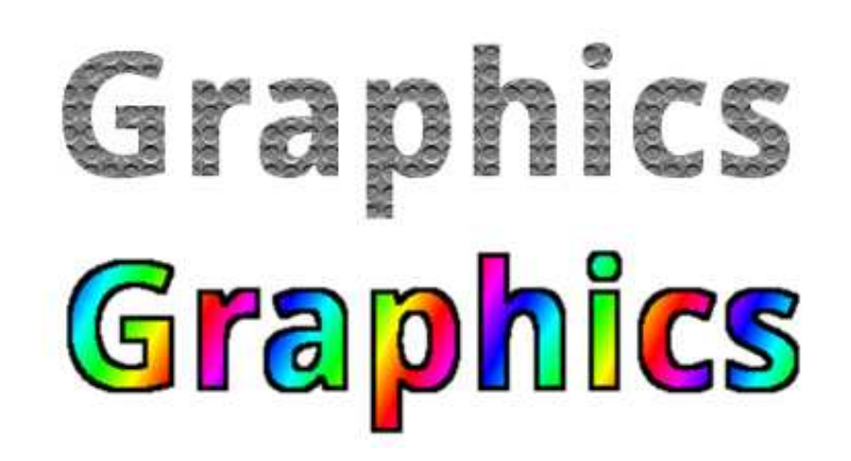
Finally, a string of text can be considered to be a shape for the purpose of drawing it. The boundary of the shape is the outline of the characters. The text is drawn by filling that shape.
In some graphics systems, it is also possible to stroke the outline of the shape that defines the text.
In the following illustration, the string "Graphics" is shown, on top, filled with a pattern and, below that, filled with a gradient and stroked with solid black:
JavaScript is a dynamic programming language that's used for web development, in web applications, for game development, and lots more. It allows we to implement dynamic features on web pages that cannot be done with only HTML and CSS.
Many browsers use JavaScript as a scripting language for doing dynamic things on the web. Any time we see a click-to-show dropdown menu, extra content added to a page, and dynamically changing element colors on a page, to name a few features, we're seeing the effects of JavaScript.
HTML defines the structure of our web document and the content therein. CSS declares various styles for the contents provided on the web document.
HTML and CSS are often called markup languages rather than programming languages, because they, at their core, provide markups for documents with very little dynamism.
JavaScript, on the other hand, is a dynamic programming language that supports Math calculations, allows we to dynamically add HTML contents to the DOM, creates dynamic style declarations, fetches contents from another website, and lots more.
Here's a basic breakdown of JavaScript fundamentals:

HTML5 (Hypertext Markup Language 5) is a markup language used for structuring and presenting hypertext documents on the World Wide Web. It was the fifth and final major HTML version that is now a retired World Wide Web Consortium (W3C) recommendation. The current specification is known as the HTML Living Standard.
Canvas is a new element in HTML5, which provides APIs used to draw raster graphics on a web application. The presence of the Canvas API for HTML5, strengthens the HTML5 platform by providing two drawing contexts: 2D and 3D. These capabilities are supported on most modern operating systems and browsers.
However, we will begin with 2D graphics.
The HTML5 canvas element is used to draw graphics, on the fly, via JavaScript. The canvas element is only a container for graphics. We must use a script to actually draw the graphics.
Canvas has several methods for drawing paths, boxes, circles, text, and adding images.
HTML Canvas can:
Here is an example of a canvas element:
<canvas id="myCanvas" width="500" height="400"></canvas>Unlike the <img> element, The <canvas> element requires the closing tag </canvas>. Any content between the opening and closing tags is fallback content that will display only if the browser doesn't support the <canvas> element.
For example:
<canvas id="myCanvas" width="500" height="400">The browser doesn't support the canvas element</canvas>However, nowadays, most modern web browsers support the <canvas> element.
Dimensions of canvas element can either be set statically in HTML, or dynamically using JavaScript, or a combination of both.
To add a border, use a style attribute:
<canvas id="myCanvas" width="500" height="400" style="border:1px solid rgb(255,0,0);"></canvas>Canvas consists of a drawable region defined in HTML code with height and width attributes. JavaScript code may access the area through a full set of drawing functions, allowing for dynamically generated graphics.
The drawing on the canvas is done with JavaScript.
The canvas is initially blank. To display something, a script is needed to access the rendering context and draw on it.
The following example draws a red rectangle on the canvas, from position (0,0) with a width of 150 and a height of 75:
Initially, the canvas is blank. To draw something, We need to access the rendering context and use it to draw on the canvas.
First, we need to find the <canvas> element.
We access a <canvas> element with the HTML DOM method getElementById():
const canvas = document.getElementById("myCanvas");The getElementById() method of the Document interface returns an Element object representing the element whose id property matches the specified string.
To set the dimensions dynamically with JavaScript, we can access the width and height as follows:
//To set width and height of current viewport
canvas.width = window.innerWidth; //or to set a specific width i.e 200
canvas.height = window.innerHeight; //or to set a specific height i.e 300Secondly, we need a drawing object for the canvas.
The getContext() method returns an object with tools (properties and methods) for drawing:
const ctx = canvas.getContext("2d");Finally, we can draw on the canvas.
Set the fill-color to red with the fillStyle property:
ctx.fillStyle = "rgb(255 0 0)";The fillStyle property can be a color, a gradient, or a pattern. The default fillStyle is black.
The fillRect(x, y, width, height) method draws the rectangle, filled with the fill style color, on the canvas:
ctx.fillRect(0, 0, 150, 75);To define fill-color and outline-color for shapes/objects in canvas, we use the following properties:
The fillStyle property defines the fill-color of the object.
The fillStyle property value can be a color (colorname, RGB, HEX, HSL), a gradient or a pattern.
const canvas = document.getElementById("myCanvas");
const ctx = canvas.getContext("2d");

//How can we set the fill-color to blue?
ctx.fillRect(10,10, 100,100);
The strokeStyle property defines the color of the outline.
The strokeStyle property value can be a color (colorname, RGB, HEX, HSL), a gradient or a pattern.
const canvas = document.getElementById("myCanvas");
const ctx = canvas.getContext("2d");

//How can we set the stroke-color to yellow?
ctx.fillRect(10,10, 100,100);It is perfectly legal to combine the previous two rectangles:
const canvas = document.getElementById("myCanvas");
const ctx = canvas.getContext("2d");

// the filled rectangle
ctx.fillStyle = "rgb(0 0 255)";
ctx.fillRect(10,10, 100,100);

// the outline rectangle
ctx.strokeStyle = "rgb(255 255 0)";
ctx.strokeRect(10,10, 100,100);
Gradients let us display smooth transitions between two or more specified colors.
Gradients can be used to fill rectangles, circles, lines, text, etc.
There are two methods used for creating gradients:
The createLinearGradient() method is used to define a linear gradient.
A linear gradient changes color along a linear pattern (horizontally/vertically/diagonally).
The createLinearGradient() method has the following parameters:
The gradient object requires two or more color stops.
The addColorStop() method specifies the color stops, and its position along the gradient. The positions can be anywhere between 0 and 1.
To use the gradient, assign it to the fillStyle or strokeStyle property, then draw the shape (rectangle, circle, shape, or text).
Here is an example of a linear gradient:
const canvas = document.getElementById("myCanvas");
const ctx = canvas.getContext("2d");

// Create gradient
const grd = ctx.createLinearGradient(0, 0, 200, 0);
grd.addColorStop(0, "red");
grd.addColorStop(1, "white");

// Fill with gradient
ctx.fillStyle = grd;
ctx.fillRect(10, 10, 150, 80);The createRadialGradient() method is used to create a radial/circular gradient.
A radial gradient is defined by two circles, one smaller and one larger.
The createRadialGradient() method has the following parameters:
Here is an example of a radial gradient:
const canvas = document.getElementById("myCanvas");

const ctx = canvas.getContext("2d");

// Create gradient
const grd2 = ctx.createRadialGradient(85, 140, 0, 85, 140, 100);

// Add color stops
grd2.addColorStop(0, "red");
grd2.addColorStop(1, "white");

// Fill with gradient
ctx.fillStyle = grd2;
ctx.fillRect(10, 100, 150, 80);
Patterns are used to fill shapes with images (instead of colors).
There are two methods used for creating patterns:
The createPattern() method has the following parameters:
Here is an example of a pattern:
const canvas = document.getElementById("myCanvas");
const ctx = canvas.getContext("2d");

// Create a pattern
const img = new Image();
img.src = "https://www.w3schools.com/tags/img_the_scream.jpg";
img.onload = function() {
  const pat = ctx.createPattern(img, "repeat");
  ctx.fillStyle = pat;
  ctx.fillRect(10, 10, 150, 80);
};
The clearRect() method is used to clear a rectangular area of the canvas. The cleared rectangle is transparent.
The clearRect() method has the following parameters:
Here we use fillRect() to draw a filled 150*100 pixels rectangle, starting in position (10,10). Then use clearRect() to clear a rectangular area in the canvas:
const canvas = document.getElementById("myCanvas");
const ctx = canvas.getContext("2d");

ctx.fillStyle = "pink";
ctx.fillRect(10,10,150,100);

ctx.clearRect(60,35,50,50);
And here is an example of clearing the entire canvas:
const canvas = document.getElementById("myCanvas");
const ctx = canvas.getContext("2d");

// Clear the canvas
ctx.clearRect(0, 0, canvas.width, canvas.height);As previously mentioned, The HTML canvas is a two-dimensional grid.
It is important to understand the coordinate space of canvas, if We want elements to be positioned as desired. Top left of canvas represents (0,0) or origin coordinate.
All the elements on canvas are placed with reference to this origin.
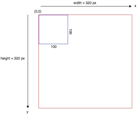
1 point on grid is roughly equivalent to 1px.
At the example above further elaborates: we have red border around our canvas and we have drawn a rectangle of 100px width and height with a stroke of blue.
This can be achieved by the following code:
<canvas id="myCanvas" width="320" height="320" style="border:1px solid rgb(255,0,0);"></canvas>const canvas = document.getElementById("myCanvas");
const ctx = canvas.getContext("2d");
ctx.strokeStyle = "rgb(0 0 255)"; //blue color for stroke
ctx.strokeRect(0, 0, 100, 100); //draws a rectangle with a blue stroke, starting at (0,0) with a width and height of 100 pixelsProviding x and y coordinates would translate the element relative to the canvas' origin coordinates.
As shown in the image below, our rectangle has moved 20 pixels to the right and bottom as we have provided the values of x and y as 20.
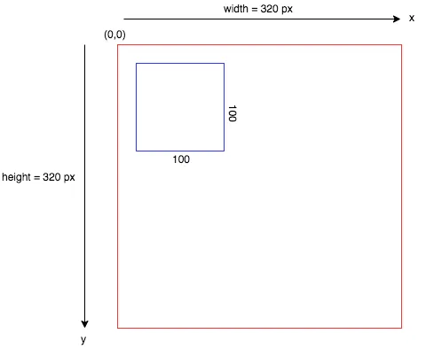
See the Pen Understanding Coordinates by Amara (@amaraauguste) on CodePen.
It is easy to draw basic shapes like rectangle, triangle, square, circle, polygon or a just a simple line between two points. But by default Canvas provides a method only to draw rectangle.
However, rest of shapes can be created by joining points using path API, and a combination of line and arc APIs.
The three most used methods for drawing rectangles in canvas are:
The rect() method defines a rectangle. Note: the rect() method does not draw the rectangle (it just defines it). So, in addition, We have to use the stroke() method (or the fill() method) to actually draw it.
fill and stroke are ink methods and each case it means to draw a rectangle with a filled color, or to draw a rectangular outline of a color. The default color is black.
ctx.fillStyle = "rgb(255 0 0)"; //red color for fill
ctx.fillRect(20, 20, 150, 100);
Here, we have drawn a red rectangle with a top-left corner at (20, 20) and a width and height of 150 and 100 pixels respectively.
Similarly, we can draw a rectangle with a stroke:
ctx.strokeStyle = "rgb(0 0 255)"; //blue color for stroke
ctx.strokeRect(20, 20, 150, 100);
Here, we have drawn a blue rectangle with a top-left corner at (20, 20) and a width and height of 150 and 100 pixels respectively.
As we mentioned earlier there is no straight forward method to create a circle, but we can use a combination of path APIs and arc method to draw our circle. Let's understand a little more about path:
"A path is list of points connected to form different shapes."
This means a path can be formed between two given points on screen. It can be a straight line or curved arc or can be any shape or color.
There are three steps to follow to create a shape using path:
Let's draw a circle:
We have to use arc(x, y, radius, startAngle, endAngle) method on context to draw our circle.
If we try to recollect basic geometry, to draw a circle using a protractor we need a radius, and a start & end angle. A semi-circle starts at angle 0 and ends at 180 degree or PI radians. So a full-circle extends further and just ends at 2*PI or 360 degrees.
This exact concept can be used to draw a circle using arc method.
ctx.beginPath(); //start a new path
ctx.arc(100, 75, 50, 0, 2 * Math.PI);
ctx.stroke();
Here, we have drawn a circle with a center at (100, 75) and a radius of 50 pixels.
To draw a half circle, we change the endAngle to PI (not 2 * PI):
ctx.beginPath(); //start a new path
ctx.arc(100, 75, 50, 0, Math.PI);
ctx.fill();The following image shows some of the angles in an arc:
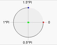
To draw a line between two points we use moveTo(x, y)and lineTo(x, y)methods.
If we consider two points A & B with x and y coordinates respectively, then moveTo acts as a position of A on canvas, while lineTo as position of point B.
ctx.beginPath();
ctx.moveTo(250, 50); //start point
ctx.lineTo(200, 100); //end point
ctx.strokeStyle = "rgb(255 105 180)"; //color of line
ctx.stroke();
The lineWidth property defines the width of the line.
It must be set before calling the stroke() method.
ctx.beginPath();
ctx.moveTo(250, 50); //start point
ctx.lineTo(200, 100); //end point
ctx.strokeStyle = "rgb(255 105 180)"; //color of line
ctx.lineWidth = 10; //width of line
ctx.stroke();A triangle is simply three lines connected together.
So, to draw a triangle we can use lineTo method to connect three points.
We are going to use a special path method called as closePath() to complete our triangle. closePath basically adds a straight line from end coordinate to the start coordinate inside a path.
If we assume a triangle is made of three points A, B & C, then we can draw our triangle like:
ctx.beginPath();
ctx.moveTo(235, 114); // Point A
ctx.lineTo(135, 349); // Point B
ctx.lineTo(335, 349); // Point C

ctx.closePath(); // Join C & A
ctx.strokeStyle = "rgb(31 24 88)";
ctx.stroke();Apart from drawing specific rectangles and circles, drawing must be broken down into four distinct steps:
In essence, We move the cursor to a starting position, tell the computer We're about to draw, record a path to a declared location, and then finally fill that path in.
To draw text on the canvas, the most important property and methods are:
The font property defines the font to be used and the size of the font. The default value for this property is "10px sans serif".
Both methods include an optional fourth parameter: maxwidth, which represents the maximum width of the text-string.
Here is an example of drawing text on a canvas:
const canvas = document.getElementById("myCanvas");
const ctx = canvas.getContext("2d");

ctx.font = "30px Arial";
ctx.fillText("Hello World", 10, 50);
The fillText() method draws filled text on the canvas. The default color of the text is black.
The strokeText() method draws text on the canvas (no fill). The default color of the text is black.
Let's take a look at some example code
Knowing what we know now about drawing shapes in Canvas
and given a canvas sized 350x350 ...
<canvas id="myCanvas" width="350" height="350" style="border:1px solid rgb(0,0,0);"></canvas>How can we can create this smiley face in the center of the canvas?
It is impossible for a graphics API to include every possible shape as a basic shape, but there is usually some way to create more complex shapes.
For example, consider polygons. A polygon is a closed shape consisting of a sequence of line segments.
Each line segment is joined to the next at its endpoint, and the last line segment connects back to the first. The endpoints are called the vertices of the polygon, and a polygon can be defined by listing its vertices.
In a regular polygon, all the sides are the same length and all the angles between sides are equal. Squares and equilateral triangles are examples of regular polygons.
A convex polygon has the property that whenever two points are inside or on the polygon, then the entire line segment between those points is also inside or on the polygon. Intuitively, a convex polygon has no "indentations" along its boundary. (Concavity can be a property of any shape, not just of polygons.)
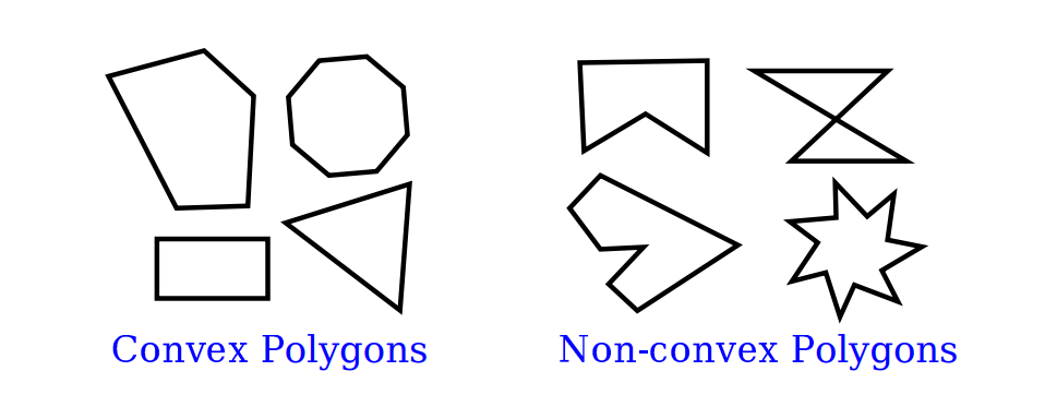
Sometimes, polygons are required to be "simple", meaning that the polygon has no selfintersections. That is, all the vertices are different, and a side can only intersect another side at its endpoints.
And polygons are usually required to be "planar", meaning that all the vertices lie in the same plane. (Of course, in 2D graphics, everything lies in the same plane, so this is not an issue. However, it does become an issue in 3D.)
How then should we draw polygons? That is, what capabilities would we like to have in a graphics API for drawing them
One possibility is to have commands for stroking and for filling polygons, where the vertices of the polygon are given as an array of points or as an array of x-coordinates plus an array of y-coordinates.
In fact, that is sometimes done; for example, the Java graphics API includes such commands.
Another, more flexible, approach is to introduce the idea of a "path."
Java, SVG, and the HTML canvas API all support this idea. A path is a general shape that can include both line segments and curved segments. Segments can, but don't have to be, connected to other segments at their endpoints.
A path is created by giving a series of commands that tell, essentially, how a pen would be moved to draw the path.
While a path is being created, there is a point that represents the pen’s current location. There will be a command for moving the pen without drawing, and commands for drawing various kinds of segments
For drawing polygons, we need commands such as:
(For closePath, I need to define “starting point.” A path can be made up of “subpaths” A subpath consists of a series of connected segments. A moveTo always starts a new subpath. A closePath ends the current segment and implicitly starts a new one. So “starting point” means the position of the pen after the most recent moveTo or closePath.)
Suppose that we want a path that represents a five sided polygon (a pentagon!).
First of all, let's consider the unit circle. This is a circle centred at (0, 0) with radius of 1 unit.
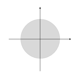
A regular polygon, such as a pentagon, can be drawn inside the unit circle as follows:
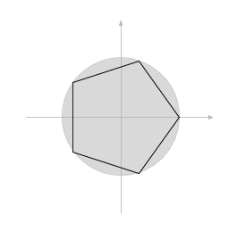
In order to draw the pentagon we need to be able to identify the 5 points on the unit circle and rotate and draw lines between them.
This is where some understanding of trigonometry comes in useful.
Let's consider some point, (a, b) on the unit circle as follows:
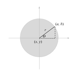
We know the radius (r), in this case it is 1 because it is the unit circle. However, it could be any length we choose.
The point (a, b) can be written in terms of trigonometric ratios as follows:
The x-coordinate is given by a = r cos 𝛳
The y-coordinate is given by b = r sin 𝛳
In Javascript we can identify the first point as:
Note that we add the (x, y) coordinate values since we will not necessarily be centering the circle at (0, 0).
Since we are drawing a pentagon we know that the angle we will need to rotate through will be 360o / 5. However, all angles must be given in radians. So the angle will be 2*Pi / 5. In Javascript this is written as:
We can now declare some variables:
We can now begin the path and set up a loop to draw each line of the polygon:
We move to the first point which is directly across from the centre of the circle (indicated in red below):
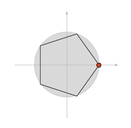
We set up a loop to draw each line and finally stroke the path when we are done.
ctx.beginPath(); // start a new path
let numberOfSides = 5; // a pentagon
let radius=100; // radius of the circle
let x = 125; // center (x) of the circle
let y = 125; // center (y)  of the circle
let angle = 2*Math.PI/numberOfSides; // angle between sides
ctx.beginPath(); // start a new path
ctx.moveTo (x + radius*Math.cos(0), y + radius*Math.sin(0)); // first vertex
for (let i = 1; i <= numberOfSides; i++) { // loop through each vertex
  ctx.lineTo (x + radius*Math.cos(i * angle), y + radius*Math.sin(i * angle)); // draw line to next vertex
}
ctx.stroke();As noted above, a path can contain other kinds of segments besides lines.
For example, it might be possible to include an arc of a circle as a segment.
Another type of curve is a Bezier curve. Bezier curves can be used to create very general curved shapes. They are fairly intuitive, so that they are often used in programs that allow users to design curves interactively.
Mathematically, Bezier curves are defined by parametric polynomial equations, but you don’t need to understand what that means to use them.
There are two kinds of Bezier curve in common use, cubic Bezier curves and quadratic Bezier curves; they are defined by cubic and quadratic polynomials respectively.
When the general term "Bezier curve" is used, it usually refers to cubic Bezier curves.
A cubic Bezier curve segment is defined by the two endpoints of the segment together with two control points. To understand how it works, it's best to think about how a pen would draw the curve segment.
The pen starts at the first endpoint, headed in the direction of the first control point. The distance of the control point from the endpoint controls the speed of the pen as it starts drawing the curve. The second control point controls the direction and speed of the pen as it gets to the second endpoint of the curve. There is a unique cubic curve that satisfies these conditions.

The illustration above shows three cubic Bezier curve segments.
The two curve segments on the right are connected at an endpoint to form a longer curve. The curves are drawn as thick black lines. The endpoints are shown as black dots and the control points as blue squares, with a thin red line connecting each control point to the corresponding endpoint. (Ordinarily, only the curve would be drawn, except in an interface that lets the user edit the curve by hand.)
Note that at an endpoint, the curve segment is tangent to the line that connects the endpoint to the control point. Note also that there can be a sharp point or corner where two curve segments meet. However, one segment will merge smoothly into the next if control points are properly chosen.
Quadratic Bezier curve segments are similar to the cubic version, but in the quadratic case, there is only one control point for the segment. The curve leaves the first endpoint heading in the direction of the control point, and it arrives at the second endpoint coming from the direction of the control point. The curve in this case will be an arc of a parabola.
The three most used methods for drawing curves in canvas are:
The quadraticCurveTo() method is used to define a quadratic Bezier curve.
The quadraticCurveTo() method has the following parameters:
Here is an example of drawing a quadratic Bezier curve:
const canvas = document.getElementById("myCanvas");
const ctx = canvas.getContext("2d");

ctx.beginPath();
ctx.moveTo(20, 100);
ctx.quadraticCurveTo(60, 10, 100, 100);
ctx.stroke();
The bezierCurveTo() method is used to define a cubic Bezier curve.
The bezierCurveTo() method has the following parameters:
Here is an example of drawing a cubic Bezier curve:
const canvas = document.getElementById("myCanvas");
const ctx = canvas.getContext("2d");

ctx.beginPath();
ctx.moveTo(20, 100);
ctx.bezierCurveTo(20, 10, 100, 10, 100, 100);
ctx.stroke();Okay, so we can draw a some shapes, lines, text, and curves. That's great and all, but how do we get from that to actually drawing on the screen with our mouse?
Since our use of Canvas is beginning to get more complex, it might help to start using functions.
Functions are a way to group together a set of instructions that perform a specific task. They allow us to reuse code, make our code more organized, and easier to read and maintain.
Let's start by creating a function that will draw a line on the canvas. We'll call this function drawLine.
function drawLine(x1, y1, x2, y2) {
  ctx.beginPath(); // Start a new path
  ctx.moveTo(x1, y1); // Move the pen to the starting point
  ctx.lineTo(x2, y2); // Draw a line to the ending point
  ctx.stroke(); // Stroke the path
}
In this function, we take four arguments: x1, y1, x2, and y2, which represent the starting and ending points of the line. We then use the canvas API to draw a line between these two points.
Now that we have our drawLine function, we can use it to draw lines on the canvas. For example:
drawLine(100, 100, 200, 200); // Draw a line from (100, 100) to (200, 200)Now, let's create a function that will draw a circle on the canvas. We'll call this function drawCircle.
function drawCircle(x, y, radius) {
  ctx.beginPath(); // Start a new path
  ctx.arc(x, y, radius, 0, Math.PI * 2); // Draw a circle
  ctx.stroke(); // Stroke the path
}
In this function, we take three arguments: x, y, and radius, which represent the center of the circle and its radius. We then use the canvas API to draw a circle at the specified location.
Now that we have our drawCircle function, we can use it to draw circles on the canvas. For example:
drawCircle(150, 150, 50); // Draw a circle with center at (150, 150) and radius of 50By creating functions like drawLine and drawCircle, we can easily draw shapes on the canvas and reuse our code to create more complex drawings.
Now that we know the structure of a basic JavaScript function, let's talk about event listeners.
Event listeners are a way to listen for and respond to events that occur in the browser. They allow us to create interactive web applications that respond to user actions such as clicks, key presses, and mouse movements.
When an event occurs, the browser triggers the event listener, which calls a function that performs a specific action. This allows us to create dynamic and interactive web pages that respond to user input.
There are many different types of events that can be listened for, such as:
Event listeners are added to elements in the DOM using the addEventListener method. This method takes two arguments: the name of the event to listen for, and the function to call when the event occurs.
For example, to listen for a click event on a button element, we can use the following code:
const button = document.getElementById('myButton'); // Get the button element
button.addEventListener('click', () => { // Listen for click event
  console.log('Button clicked!'); // Log a message to the console
});
Let's add a button to clear the canvas:
First, let's create a new canvas and a button:
<canvas id="myCanvas" width="500" height="400" style="border:1px solid #000000;"></canvas>
<button id="clearButton">Clear Canvas</button>
Next, let's add an event listener to the button that clears the canvas:
const canvas = document.getElementById('myCanvas'); // Get the canvas element
const ctx = canvas.getContext('2d'); // Get the 2D drawing context

const clearButton = document.getElementById('clearButton'); // Get the clear button element

clearButton.addEventListener('click', () => { // Listen for click event on clear button
  ctx.clearRect(0, 0, canvas.width, canvas.height); // Clear the canvas
});
In this example, we get the canvas element and its 2D drawing context, as well as the clear button element. We then add an event listener to the clear button that calls the clearRect method on the canvas context to clear the canvas when the button is clicked.
So let's draw some shapes on the canvas:
drawLine(100, 100, 200, 200); // Draw a line from (100, 100) to (200, 200)
drawCircle(150, 150, 50); // Draw a circle with center at (150, 150) and radius of 50
And now we can clear the canvas!
So far, we've used JavaScript to draw shapes on the canvas and an event listener to add button functionalty to clear the canvas, but that's not really how we draw, is it?
A good drawing application has to respond to the mouse. We need to be able to draw lines and shapes by clicking and dragging the mouse.
We need a listener that responds to the canvas being clicked, and another listener that responds to mouse movement, but only when the mouse button is pressed down.
Mouse events in JavaScript allow us to create interactive and dynamic web applications. By capturing mouse events, we can respond to user actions such as clicks, movements, and drags. This is particularly useful when working with the HTML5 canvas element, as it enables us to create drawing applications, games, and other interactive graphics.
JavaScript provides several mouse events that we can listen for:
To use mouse events with the HTML5 canvas, we need to add event listeners to the canvas element. These event listeners will call functions that handle the events and perform actions such as drawing on the canvas.
To determine the mouse position within the canvas, we need to account for the canvas's position relative to the viewport. This can be done using the getBoundingClientRect() method, which returns the size of an element and its position relative to the viewport.
Here is an example of how to determine the mouse position within the canvas:
function getMousePos(canvas, event) {
const rect = canvas.getBoundingClientRect(); // Get the size and position of the canvas
  return {
    x: event.clientX - rect.left, // X coordinate of mouse relative to canvas
    y: event.clientY - rect.top // Y coordinate of mouse relative to canvas
  };
}

// Example usage
canvas.addEventListener('mousemove', (event) => { // Listen for mousemove event
  const mousePos = getMousePos(canvas, event); // Get the mouse position
  console.log('Mouse position: ' + mousePos.x + ',' + mousePos.y); // Log the mouse position
});
In this example:
Now let's try using the mouse to draw.
<canvas id="myCanvas" width="500" height="400" style="border:1px solid #000000;"></canvas>const canvas = document.getElementById('myCanvas');
const ctx = canvas.getContext('2d');
let painting = false; // Flag to indicate if the user is drawing
function startPosition(e) {
painting = true;
draw(e);
}
function endPosition() {
painting = false;
ctx.beginPath(); // Begin a new path to avoid connecting lines
}
function draw(e) {
if (!painting) return; // Exit the function if the user is not drawing
ctx.lineWidth = 5; // Set the line width
ctx.strokeStyle = 'black'; // Set the line color
ctx.lineTo(e.clientX - canvas.offsetLeft, e.clientY - canvas.offsetTop); // Draw a line to the current mouse position
ctx.stroke(); // Stroke the line
ctx.beginPath(); // Begin a new path
ctx.moveTo(e.clientX - canvas.offsetLeft, e.clientY - canvas.offsetTop); // Move to the new starting point
}
canvas.addEventListener('mousedown', startPosition); // Listen for mousedown event
canvas.addEventListener('mouseup', endPosition); // Listen for mouseup event
canvas.addEventListener('mousemove', draw);In this example:
In another example we can use our mouse to draw circles on the canvas:
const canvas = document.getElementById('myCanvas');
const ctx = canvas.getContext('2d');
let painting = false; // Flag to indicate if the user is drawing

function drawCircle(e) {
  if (!painting) return; // Exit the function if the user is not drawing

  ctx.beginPath(); // Start a new path
  ctx.arc(e.clientX - canvas.offsetLeft, e.clientY - canvas.offsetTop, 10, 0, Math.PI * 2); // Draw a circle
  ctx.fill(); // Fill the circle
}

canvas.addEventListener('mousedown', (e) => { // Listen for mousedown event
  painting = true; // Set the painting flag to true
  drawCircle(e); // Draw a circle
});

canvas.addEventListener('mouseup', () => { // Listen for mouseup event
  painting = false; // Set the painting flag to false
});

canvas.addEventListener('mousemove', drawCircle); // Listen for mousemove event
In this example:
We can simplify the code a bit by using getBoundingClientRect which gives the size of an element and its position relative to the viewport:
const canvas = document.getElementById('myCanvas');
const ctx = canvas.getContext('2d');

ctx.beginPath(); // Start a new path
ctx.arc(e.clientX - canvas.getBoundingClientRect().left, e.clientY - canvas.getBoundingClientRect().top, 10, 0, Math.PI * 2); // Draw a circle
ctx.fill(); // Fill the circle
Although this works, we can achieve the same result a bit simpler with offsetX and offsetY:
const canvas = document.getElementById('myCanvas');
const ctx = canvas.getContext('2d');

canvas.addEventListener('mousedown', (e) => { // Listen for mousedown event
ctx.beginPath(); // Start a new path
ctx.arc(e.offsetX, e.offsetY, 10, 0, Math.PI * 2); // Draw a circle
ctx.fill(); // Fill the circle
});
This works because offsetX and offsetY give the position of the mouse relative to the target element, in this case the canvas.
So to rewrite our draw function:
function draw(e) {
    if (!painting) return; // Exit the function if the user is not drawing

    ctx.lineWidth = 5; // Set the line width
    ctx.strokeStyle = 'black'; // Set the line color

    ctx.lineTo(e.offsetX, e.offsetY); // Draw a line to the current mouse position
    ctx.stroke(); // Stroke the line
    ctx.beginPath(); // Begin a new path
    ctx.moveTo(e.offsetX, e.offsetY); // Move to the new starting point
}
And that's it! We can now draw on the canvas with our mouse.
By combining mouse events with the canvas API, we can create interactive drawing applications that respond to user input.
How can we draw the following graphics on a 400 x 400 canvas?
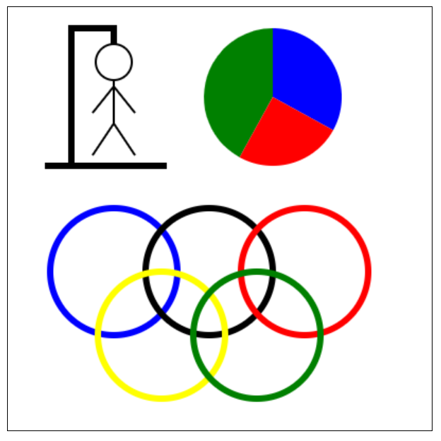
In addition to our mouse down events, there are also a few others that may come in handy (for both 2D and 3D graphics)
Keyboard events are triggered when a key is pressed or released on the keyboard. They allow us to respond to user input and create interactive web applications that respond to key presses.
There are several keyboard events that we can listen for:
Keyboard events provide information about the key that was pressed, such as the key code and the key value. This information can be used to perform specific actions based on the key that was pressed.
Here is an example of how to listen for keyboard events:
document.addEventListener('keydown', (event) => { // Listen for keydown event
  console.log('Key pressed: ' + event.key); // Log the key that was pressed

  if (event.key == 'ArrowUp') {
    console.log('Up arrow key pressed'); // Log a message if the up arrow key was pressed
  }

  if (event.key == 'ArrowDown') {
    console.log('Down arrow key pressed'); // Log a message if the down arrow key was pressed
  }

  // Add more key press conditions as needed
});
Each key on the keyboard has a unique key code and key value. The key code is a numerical value that represents the key, while the key value is a string that represents the key.
For example, the key code for the up arrow key is 38, and the key value is 'ArrowUp'.
Standard key codes are as follows:
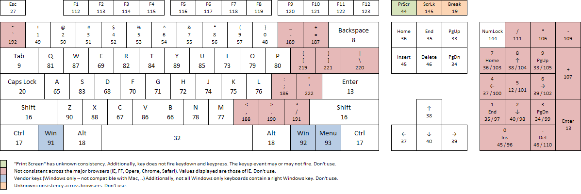
Keyboard events can be used to create keyboard shortcuts, control game characters, and more.
For example, let's write some code to create a rectangle that we will be able to move with the WASD and directional arrow keys:
const canvas = document.getElementById('myCanvas');
const ctx = canvas.getContext('2d');
let x = 100; // Initial x position of the rectangle
let y = 100; // Initial y position of the rectangle
let speed = 5; // Speed of the rectangle

function drawRectangle() {
    ctx.clearRect(0, 0, canvas.width, canvas.height); // Clear the canvas
    ctx.fillStyle = 'blue'; // Set rectangle color
    ctx.fillRect(x, y, 50, 50); // Draw the rectangle
}

document.addEventListener('keydown', (event) => { // Listen for keydown event
    switch (event.key) {
        case 'ArrowUp':
        case 'w':
            y -= speed; // Move the rectangle up
            break;
        case 'ArrowDown':
        case 's':
            y += speed; // Move the rectangle down
            break;
        case 'ArrowLeft':
        case 'a':
            x -= speed; // Move the rectangle left
            break;
        case 'ArrowRight':
        case 'd':
            x += speed; // Move the rectangle right
            break;
    }

    drawRectangle(); // Redraw the rectangle
});

// Initial call to draw the rectangle when the page loads
drawRectangle();
In this example:
In the early days of touch-enabled devices, touch events were often interpreted and essentially "translated" into mouse events for compatibility with existing web applications, meaning that a touch interaction would trigger a corresponding mouse event like a click or hover, although this approach had limitations when dealing with multi-touch gesture.
With the widespread adoption of touchscreen devices, such as a smartphone or tablet, HTML5 brings to the table, among many other things, a set of touch-based interaction events.
Mouse-based events such as hover, mouse in, mouse out etc. aren't able to adequately capture the range of interactions possible via touchscreen, so touch events are a welcome and necessary addition to the web developer's toolbox.
They allow us to create web applications that respond to touch gestures, such as tapping, swiping, and pinching.
Use cases for the touch events API include gesture recognition, multi-touch, drag and drop, and any other touch-based interfaces.
We'll get some of the technical details of the API out of the way first, before moving on to some real examples. The API is defined in terms of Touches, TouchEvents, and TouchLists.
Each Touch describes a touch point, and has the following attributes:
There are several touch events that we can listen for:
Touch events provide information about the touch points, such as the touch coordinates and the touch identifier. This information can be used to perform specific actions based on the touch gestures.
Here is an example of how to listen for touch events:
document.addEventListener('touchstart', (event) => { // Listen for touchstart event
  console.log('Touch started at: ' + event.touches[0].clientX + ',' + event.touches[0].clientY); // Log the touch
  coordinates
});
Let's go one step further and display the touch position information visually, by displaying a dot on the canvas at the point where it was touched.
const canvas = document.getElementById('myCanvas');
const ctx = canvas.getContext('2d');

canvas.addEventListener('touchstart', (event) => { // Listen for touchstart event
  const touch = event.touches[0]; // Get the first touch point
  const x = touch.clientX - canvas.offsetLeft; // Calculate the x-coordinate relative to the canvas
  const y = touch.clientY - canvas.offsetTop; // Calculate the y-coordinate relative to the canvas

  ctx.beginPath(); // Start a new path
  ctx.arc(x, y, 5, 0, Math.PI * 2); // Draw a circle at the touch point
  ctx.fill(); // Fill the circle
});
In this example:
Touch events are widely supported among mobile devices.
However, unless specifically targeting touch devices, a fallback should be implemented when touchevents are not supported. In these cases, the traditional click etc. events can be bound to, but as discussed below, care is needed when deciding which events to support instead of the touch events.
Since touch events may not be supported on a user's device - indeed, the user may not even be accessing your app on a touchscreen device - this contingency should be planned for.
You may want to enable your app to support particular mouse events instead. Care should be taken here as there is not a one-to-one correspondance between mouse events and touch events, and the behaviour differences can be subtle.
So for our code we should also enable mouse events:
canvas.addEventListener('mousedown', (event) => { // Listen for mousedown event
const x = event.clientX - canvas.offsetLeft; // Calculate the x-coordinate relative to the canvas
const y = event.clientY - canvas.offsetTop; // Calculate the y-coordinate relative to the canvas

ctx.beginPath(); // Start a new path
ctx.arc(x, y, 5, 0, Math.PI * 2); // Draw a circle at the mouse point
ctx.fill(); // Fill the circle
});Care should also be taken implementing touch events that the events don't interfere with typical browser behaviours such as scrolling and zooming - thus there is an argument for disabling these default browser behaviours if you are making use of touch events.
It is also important to remember that touch events are not the same as mouse events.
For example, a touchstart event is not the same as a mousedown event. The former is triggered when a touch point is placed on the touch surface, while the latter is triggered when a mouse button is pressed down.
Therefore, it is important to consider the differences between touch and mouse events when designing touch-based interfaces.
Finally, it is important to test touch events on a variety of devices to ensure that they work as expected and provide a good user experience.
In addition, there are also scroll events, resize events, and more. These can all be used to create more interactive and dynamic web applications.
It is possible to transform coordinates from one coordinate system to another. Let's look at how geometric transformations can be used to place graphics objects into a coordinate system.
In a typical application, we have a rectangle made of pixels, with its natural pixel coordinates, where an image will be displayed. This rectangle will be called the viewport.
We also have a set of geometric objects that are defined in a possibly different coordinate system, generally one that uses real-number coordinates rather than integers. These objects make up the “scene” or "world" that we want to view, and the coordinates that we use to define the scene are called world coordinates.
For 2D graphics, the world lies in a plane. It's not possible to show a picture of the entire infinite plane. We need to pick some rectangular area in the plane to display in the image. Let's call that rectangular area the window, or view window.
A coordinate transform is used to map the window to the viewport.
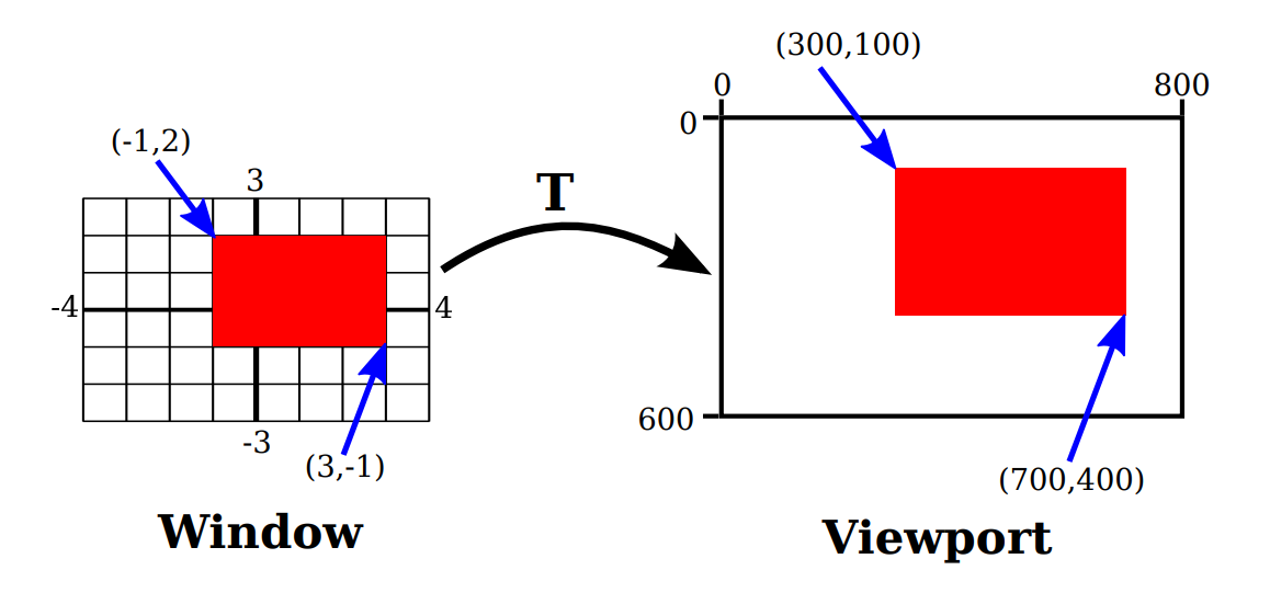
In this illustration, T represents the coordinate transformation. T is a function that takes world coordinates (x,y) in some window and maps them to pixel coordinates T(x,y) in the viewport
In this example, as you can check,
Look at the rectangle with corners at (-1,2) and (3,-1) in the window. When this rectangle is displayed in the viewport, it is displayed as the rectangle with corners T(-1,2) and T(3,-1). In this example, T(-1,2) = (300,100) and T(3,-1) = (700,400).
We use coordinate transformations in this way because it allows us to choose a world coordinate system that is natural for describing the scene that we want to display, and it is easier to do that than to work directly with viewport coordinates. Along the same lines, suppose that we want to define some complex object, and suppose that there will be several copies of that object in our scene. Or maybe we are making an animation, and we would like the object to have different positions in different frames.
We would like to choose some convenient coordinate system and use it to define the object once and for all.
The coordinates that we use to define an object are called object coordinates for the object.
When we want to place the object into a scene, we need to transform the object coordinates that we used to define the object into the world coordinate system that we are using for the scene. The transformation that we need is called a modeling transformation.
This picture illustrates an object defined in its own object coordinate system and then mapped by three different modeling transformations into the world coordinate system:
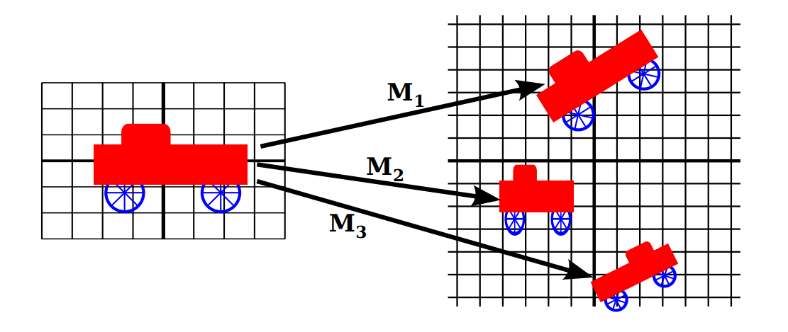
Remember that in order to view the scene, there will be another transformation that maps the object from a view window in world coordinates into the viewport.
Now, keep in mind that the choice of a view window tells which part of the scene is shown in the image. Moving, resizing, or even rotating the window will give a different view of the scene. Suppose we make several images of the same car:
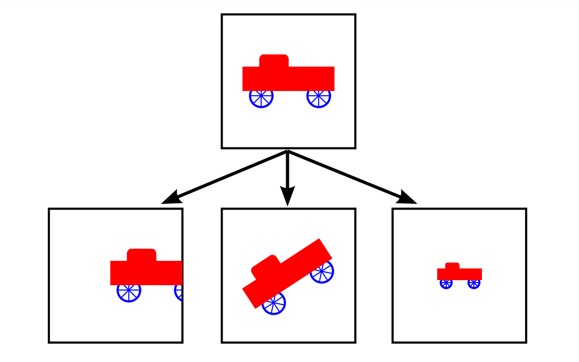
What happened between making the top image in this illustration and making the image on the bottom left?
In fact, there are two possibilities: Either the car was moved to the right, or the view window that defines the scene was moved to the left.
This is important, so be sure you understand it. (Try it with your cell phone camera. Aim it at some objects, take a step to the left, and notice what happens to the objects in the camera's viewfinder: They move to the right in the picture!)
Similarly, what happens between the top picture and the middle picture on the bottom? Either the car rotated counterclockwise, or the window was rotated clockwise. (Again, try it with a camera—you might want to take two actual photos so that you can compare them.)
Finally, the change from the top picture to the one on the bottom right could happen because the car got smaller or because the window got larger. (On your camera, a bigger window means that you are seeing a larger field of view, and you can get that by applying a zoom to the camera or by backing up away from the objects that you are viewing.)
There is an important general idea here. When we modify the view window, we change the coordinate system that is applied to the viewport. But in fact, this is the same as leaving that coordinate system in place and moving the objects in the scene instead. Except that to get the same effect in the final image, you have to apply the opposite transformation to the objects (for example, moving the window to the left is equivalent to moving the objects to the right).
So, there is no essential distinction between transforming the window and transforming the object. Mathematically, you specify a geometric primitive by giving coordinates in some natural coordinate system, and the computer applies a sequence of transformations to those coordinates to produce, in the end, the coordinates that are used to actually draw the primitive in the image.
You will think of some of those transformations as modeling transforms and some as coordinate transforms, but to the computer, it's all the same.
We will return to this idea several times later throughout this class, but in any case, you can see that geometric transforms are a central concept in computer graphics. Let's look at some basic types of transformation in more detail.
The transforms we will use in 2D graphics can be written in the form:
where (x,y) represents the coordinates of some point before the transformation is applied, and (x1,y1 ) are the transformed coordinates.
The transform is defined by the six constants a, b, c, d, e, and f. Note that this can be written as a function T, where
A transformation of this form is called an affine transform.
An affine transform has the property that, when it is applied to two parallel lines, the transformed lines will also be parallel. Also, if you follow one affine transform by another affine transform, the result is again an affine transform.
There are four basic types of affine transforms that are commonly used in computer graphics:
A translation transform simply moves every point by a certain amount horizontally and a certain amount vertically.
If (x,y) is the original point and (x1,y1) is the transformed point, then the formula for a translation is:
where e is the number of units by which the point is moved horizontally and f is the amount by which it is moved vertically. (Thus for a translation, a = d = 1, and b = c = 0 in the general formula for an affine transform.)
A 2D graphics system will typically have a function such as:
to apply a translate transformation. The translation would apply to everything that is drawn after the command is given. That is, for all subsequent drawing operations, e would be added to the x-coordinate and f would be added to the y-coordinate.
Let's look at an example: Suppose that you draw an "F" using coordinates in which the "F" is centered at (0,0).
If you say translate(4,2) before drawing the "F", then every point of the "F" will be moved horizontally by 4 units and vertically by 2 units before the coordinates are actually used, so that after the translation, the "F" will be centered at (4,2):
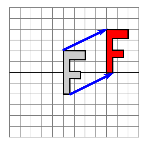
The light gray "F" in this picture shows what would be drawn without the translation; the dark red "F" shows the same "F" drawn after applying a translation by (4,2).
The top arrow shows that the upper left corner of the "F" has been moved over 4 units and up 2 units. Every point in the "F" is subjected to the same displacement.
Note that in these examples, we are assuming that the y-coordinate increases from bottom to top. That is, the y-axis points up.
Remember that when you give the command translate(e,f), the translation applies to all the drawing that you do after that, not just to the next shape that you draw.
If you apply another transformation after the translation, the second transform will not replace the translation. It will be combined with the translation, so that subsequent drawing will be affected by the combined transformation.
For example, if you combine translate(4,2) with translate(-1,5), the result is the same as a single translation, translate(3,7). This is an important point, and there will be a lot more to say about it later.
Also remember that you don't compute coordinate transformations yourself. You just specify the original coordinates for the object (that is, the object coordinates), and you specify the transform or transforms that are to be applied. The computer takes care of applying the transformation to the coordinates.
You don't even need to know the exact equations that are used for the transformation; you just need to understand what it does geometrically.
HTML5 Canvas has a built in translate() method - used to move an object by x and y, where:
For example, here is how you might use the translate function in HTML5 Canvas:
First, draw one rectangle in position (10,10), then set translate() to (70,70) (This will be the new start point). Then draw another rectangle in position (10,10). Notice that the second rectangle now starts in position (80,80):
const canvas = document.getElementById("myCanvas");
const ctx = canvas.getContext("2d");

ctx.fillStyle = "red";
ctx.fillRect(10, 10, 100, 50);

ctx.translate(70, 70);

ctx.fillStyle = "blue";
ctx.fillRect(10, 10, 100, 50);
Our first rectangle is placed at position (10, 10) but when we use translate(70,70), even though our next drawn rectangle is also placed at position (10, 10), it is actually placed at position (80, 80) because our x-position is now (70 + 10) and y-position is now (70 + 10).
A rotation transform, for our purposes here, rotates each point about the origin, (0,0). Every point is rotated through the same angle, called the angle of rotation.
For this purpose, angles can be measured either in degrees or in radians.
A rotation with a positive angle rotates objects in the direction from the positive x-axis towards the positive y-axis.
This is counterclockwise in a coordinate system (cartesian) where the y-axis points up, as it does in my examples here, but it is clockwise in the usual pixel coordinates, where the y-axis points down rather than up.
Although it is not obvious, when rotation through an angle of r radians about the origin is applied to the point (x,y), then the resulting point (x1,y1 ) is given by:
That is, in the general formula for an affine transform, e = f = 0, a = d = cos(r), b = -sin(r), and c = sin(r).
Here is a picture that illustrates a rotation about the origin by the angle negative 135 degrees:
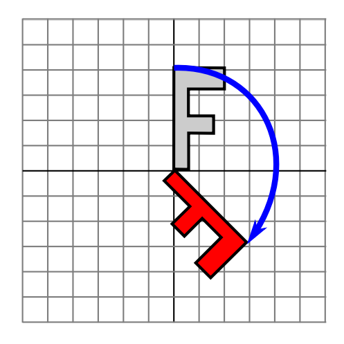
Again, the light gray "F" is the original shape, and the dark red "F" is the shape that results if you apply the rotation. The arrow shows how the upper left corner of the original “F” has been moved.
A 2D graphics API would typically have a command rotate(r) to apply a rotation. The command is used before drawing the objects to which the rotation applies.
For example, HTML5 Canvas has a rotate method that takes an angle in radians as a parameter. The rotation is applied to all subsequent drawing operations.
As a reminder, angles are in radians, as opposed to degrees. So we use (Math.PI/180)*[degree] to convert.
Let's rotate a rectangle in canvas:
const canvas = document.getElementById("myCanvas");
const ctx = canvas.getContext("2d");

ctx.fillStyle = "red";
ctx.fillRect(50, 10, 100, 50);

ctx.rotate((Math.PI/180)*20); // Rotate 20 degrees

ctx.strokeStyle = "blue";
ctx.strokeRect(70, 30, 100, 50);
Remember that the rotation is applied to all subsequent drawing operations, so we need to translate to the center of the rectangle to rotate it around its center.
A scaling transform can be used to make objects bigger or smaller.
Mathematically, a scaling transform simply multiplies each x-coordinate by a given amount and each y-coordinate by a given amount.
That is, if a point (x,y) is scaled by a factor of a in the x direction and by a factor of d in the y direction, then the resulting point (x1,y1 ) is given by:
If you apply this transform to a shape that is centered at the origin, it will stretch the shape by a factor of a horizontally and d vertically.
Here is an example, in which the original light gray "F" is scaled by a factor of 3 horizontally and 2 vertically to give the final dark red "F":
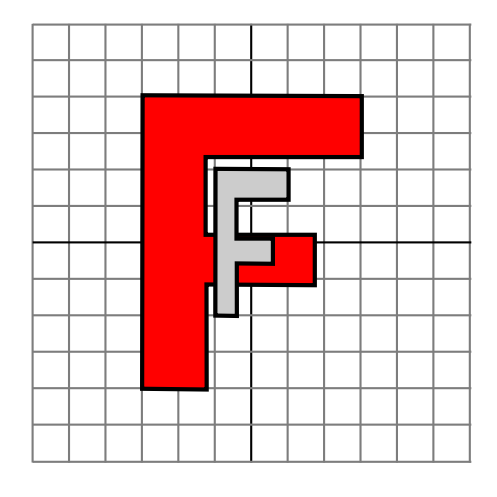
The common case where the horizontal and vertical scaling factors are the same is called uniform scaling. Uniform scaling stretches or shrinks a shape without distorting it.
When scaling is applied to a shape that is not centered at (0,0), then in addition to being stretched or shrunk, the shape will be moved away from 0 or towards 0. In fact, the true description of a scaling operation is that it pushes every point away from (0,0) or pulls every point towards (0,0). If you want to scale about a point other than (0,0), you can use a sequence of three transforms, similar to what was done in the case of rotation.
A 2D graphics API can provide a function scale(a,d) for applying scaling transformations. As usual, the transform applies to all x and y coordinates in subsequent drawing operations.
One unit on the canvas is one pixel. If we set the scaling factor to 2, one unit becomes two pixels, and shapes will be drawn twice as large. If we set a scaling factor to 0.5, one unit becomes 0.5 pixels, and shapes will be drawn at half size.
Note that negative scaling factors are allowed and will result in reflecting the shape as well as possibly stretching or shrinking it. For example, scale(1,-1) will reflect objects vertically, through the x -axis.
As with the other transformations, a scaling transform is applied to all subsequent drawing operations. In HTML5 Canvas, you can use the scale method to apply a scaling transform:
The scale() method has the following parameters:
One unit on the canvas is one pixel.
So, if we set the scaling factor to 2, one unit becomes two pixels, and shapes will be drawn twice as large. If we set a scaling factor to 0.5, one unit becomes 0.5 pixels, and shapes will be drawn at half size.
const canvas = document.getElementById("myCanvas");
const ctx = canvas.getContext("2d");

ctx.strokeRect(5, 5, 100, 75);

ctx.scale(2, 2);

ctx.strokeStyle = "blue";
ctx.strokeRect(5, 5, 100, 75);
It is a fact that every affine transform can be created by combining translations, rotations about the origin, and scalings about the origin.
Also note that a transform that is made from translations and rotations, with no scaling, will preserve length and angles in the objects to which it is applied. It will also preserve aspect ratios of rectangles.
Transforms with this property are called "Euclidean". If you also allow uniform scaling, the resulting transformation will preserve angles and aspect ratio, but not lengths.
We will look at one more type of basic transform, a shearing transform.
Although shears can in fact be built up out of rotations and scalings if necessary, it is not really obvious how to do so.
A shear will "tilt" objects. A horizontal shear will tilt things towards the left (for negative shear) or right (for positive shear). A vertical shear tilts them up or down.
Here is an example of horizontal shear:
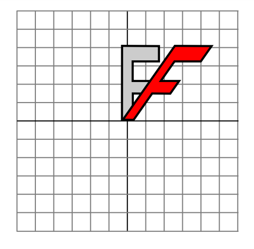
A horizontal shear does not move the x-axis. Every other horizontal line is moved to the left or to the right by an amount that is proportional to the y-value along that line.
When a horizontal shear is applied to a point (x,y), the resulting point (x1,y1) is given by:
for some constant shearing factor b. Similarly, a vertical shear with shearing factor c is given by the equations:
Shear is occasionally called "skew", but skew is usually specified as an angle rather than as a shear factor.
As we just saw, we are now in a position to see what can happen when you combine two transformations. Suppose that before drawing some object, you say:
Assume that angles are measured in degrees.
The translation will then apply to all subsequent drawing. But, because of the rotation command, the things that you draw after the translation are rotated objects.
That is, the translation applies to objects that have already been rotated.
An example is shown on the left in the illustration below, where the light gray "F" is the original shape, and red "F" shows the result of applying the two transforms to the original.
The original "F" was first rotated through a 90 degree angle, and then moved 4 units to the right.
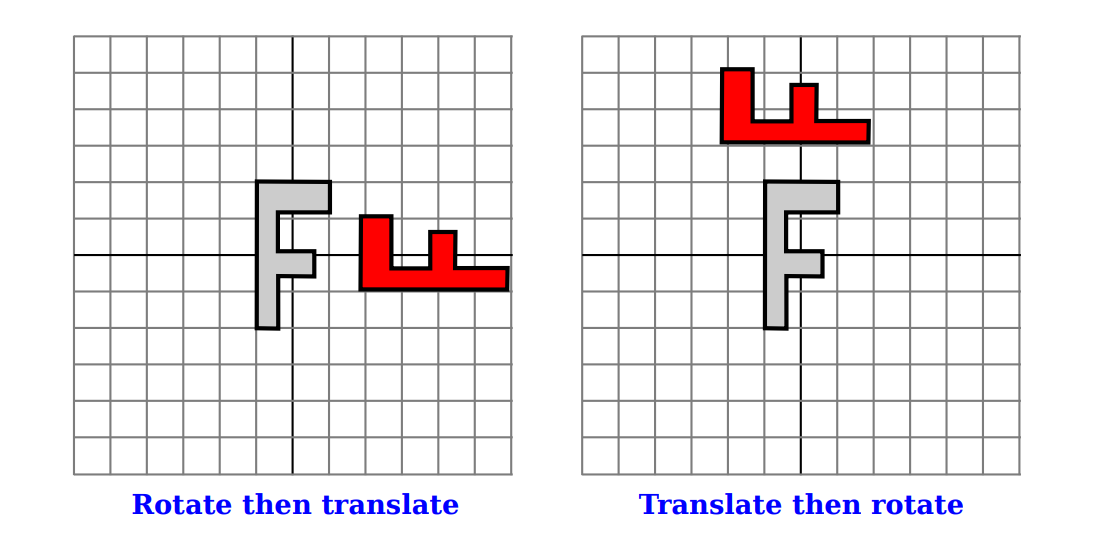
Note that transforms are applied to objects in the reverse of the order in which they are given in the code (because the first transform in the code is applied to an object that has already been affected by the second transform). And note that the order in which the transforms are applied is important.
If we reverse the order in which the two transforms are applied in this example, by saying:
then the result is as shown on the right in the above illustration. In that picture, the original "F" is first moved 4 units to the right and the resulting shape is then rotated through an angle of 90 degrees about the origin to give the shape that actually appears on the screen.
For another example of applying several transformations, suppose that we want to rotate a shape through an angle r about a point (p,q) instead of about the point (0,0).
We can do this by first moving the point (p,q) to the origin, using translate(-p,-q). Then we can do a standard rotation about the origin by calling rotate(r). Finally, we can move the origin back to the point (p,q) by applying translate(p,q).
Keeping in mind that we have to write the code for the transformations in the reverse order, we need to say:
before drawing the shape. (In fact, some graphics APIs let us accomplish this transform with a single command such as rotate(r,p,q). This would apply a rotation through the angle r about the point (p,q).)
In HTML5 Canvas, we have a method called transform().
The transform() method replaces the current transformation matrix with the matrix described by the arguments of this method. The transform() method multiplies the current transformation matrix with the matrix described by the arguments of this method. This is useful for applying multiple transformations to the same shape.
The transform method takes the following parameters:
Here is an example of how to use the transform() method in HTML5 Canvas:
const canvas = document.getElementById("myCanvas");
const ctx = canvas.getContext("2d");

ctx.strokeRect(5, 5, 100, 75);

ctx.transform(2, 0, 0, 2, 40, 40); // Scale by 2 and move 40 units
ctx.strokeStyle = "blue";
ctx.strokeRect(5, 5, 100, 75);
We can scale, rotate, and translate using a mixture of these methods as well:
const canvas = document.getElementById("myCanvas");
const ctx = canvas.getContext("2d");

ctx.strokeRect(5, 5, 100, 75);

ctx.translate(200, 40); // Move 200 units to the right and 40 units down
ctx.rotate((Math.PI/180)*45); // Rotate 45 degrees
ctx.scale(2, 2); // Scale by 2

ctx.strokeStyle = "blue";
ctx.strokeRect(5, 5, 100, 75);
Note that we will talk again about transformations in the context of 3D graphics, where they become even more important.
Linear algebra is a branch of mathematics that deals with vectors and matrices. It is a fundamental tool in computer graphics, as it allows us to perform transformations on objects in 2D and 3D space.
A vector is a quantity that has a length and a direction.
A vector can be visualized as an arrow, as long as you remember that it is the length and direction of the arrow that are relevant, and that its specific location is irrelevant.
Vectors are often used in computer graphics to represent directions, such as the direction from an object to a light source or the direction in which a surface faces. In those cases, we are more interested in the direction of a vector than in its length.
If we visualize a 3D vector V as an arrow starting at the origin, (0,0,0), and ending at a point P, then we can, to a certain extent, identify V with P—at least as long as we remember that an arrow starting at any other point could also be used to represent V. If P has coordinates (a,b,c), we can use the same coordinates for V.
When we think of (a,b,c) as a vector, the value of a represents the change in the x -coordinate between the starting point of the arrow and its ending point, b is the change in the y-coordinate, and c is the change in the z -coordinate. For example, the 3D point (x,y,z ) = (3,4,5) has the same coordinates as the vector (dx,dy,dz ) = (3,4,5).
For the point, the coordinates (3,4,5) specify a position in space in the xyz coordinate system.
For the vector, the coordinates (3,4,5) specify the change in the x, y, and z coordinates along the vector.
If we represent the vector with an arrow that starts at the origin (0,0,0), then the head of the arrow will be at (3,4,5). But we could just as well visualize the vector as an arrow that starts at the point (1,1,1), and in that case the head of the arrow would be at the point (4,5,6).
The distinction between a point and a vector is subtle. For some purposes, the distinction can be ignored; for other purposes, it is important. Often, all that we have is a sequence of numbers, which we can treat as the coordinates of either a vector or a point, whichever is more appropriate in the context.
One of the basic properties of a vector is its length. In terms of its coordinates, the length of a 3D vector (x,y,z) is given by sqrt(x^2+y^2+z^2). (This is just the Pythagorean theorem in three dimensions.) If v is a vector, its length is denoted by |v|.
The length of a vector is also called its norm. (We are considering 3D vectors here, but concepts and formulas are similar for other dimensions.)
Vectors of length 1 are particularly important. They are called unit vectors. If v = (x,y,z ) is any vector other than (0,0,0), then there is exactly one unit vector that points in the same direction as v.
That vector is given by:
where length is the length of v. Dividing a vector by its length is said to normalize the vector: The result is a unit vector that points in the same direction as the original vector.
Two vectors can be added. Given two vectors v1 = (x1,y1,z1) and v2 = (x2,y2,z2), their sum is defined as:
The sum has a geometric meaning:

Multiplication is more complicated. The obvious definition of the product of two vectors, similar to the definition of the sum, does not have geometric meaning and is rarely used.
However, there are three kinds of vector multiplication that are used: the scalar product, the dot product, and the cross product.
If v = (x,y,z ) is a vector and a is a number, then the scalar product of a and v is defined as:
Assuming that a is positive and v is not zero, av is a vector that points in the same direction as v, whose length is a times the length of v. If a is negative, av points in the opposite direction from v, and its length is |a| times the length of v.
This type of product is called a scalar product because a number like a is also referred to as a "scalar", perhaps because multiplication by a scales v to a new length.
Given two vectors v1 = (x1,y1,z1 ) and v2 = (x2,y2,z2 ), the dot product of v1 and v2 is denoted by v1 ·v2 and is defined by:
Note that the dot product is a number, not a vector.
The dot product has several very important geometric meanings. First of all, note that the length of a vector v is just the square root of v·v. Furthermore, the dot product of two non-zero vectors v1 and v2 has the property that:
where angle is the measure of the angle between v1 and v2.
In particular, in the case of two unit vectors, whose lengths are 1, the dot product of two unit vectors is simply the cosine of the angle between them.
Furthermore, since the cosine of a 90-degree angle is zero, two non-zero vectors are perpendicular if and only if their dot product is zero. Because of these properties, the dot product is particularly important in lighting calculations, where the effect of light shining on a surface depends on the angle that the light makes with the surface.
The scalar product and dot product are defined in any dimension.
For vectors in 3D, there is another type of product called the cross product, which also has an important geometric meaning. For vectors v1 = (x1,y1,z1) and v2 = (x2,y2,z2), the cross product of v1 and v2 is denoted v1×v2 and is the vector defined by:
If v1 and v2 are non-zero vectors, then v1×v2 is zero if and only if v1 and v2 point in the same direction or in exactly opposite directions.
Assuming v1×v2 is non-zero, then it is perpendicular both to v1 and to v2 ; furthermore, the vectors v1, v2, v1×v2 follow the right-hand rule (in a right-handed coordinate system); that is, if you curl the fingers of your right hand from v1 to v2, then your thumb points in the direction of v1×v2.
If v1 and v2 are perpendicular unit vectors, then the cross product v1×v2 is also a unit vector, which is perpendicular both to v1 and to v2.
Finally, I will note that given two points P1 = (x1,y1,z1 ) and P2 = (x2,y2,z2 ), the difference P2−P1 is defined by:
This difference is a vector that can be visualized as an arrow that starts at P1 and ends at P2.
Now, suppose that P1, P2, and P3 are vertices of a polygon. Then the vectors P1−P2 and P3−P2 lie in the plane of the polygon, and so the cross product:
is a vector that is perpendicular to the polygon.
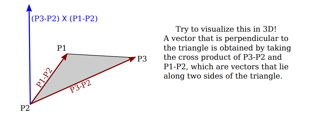
This vector is said to be a normal vector for the polygon.
A normal vector of length one is called a unit normal. Unit normals will be important in lighting calculations, and it will be useful to be able to calculate a unit normal for a polygon from its vertices.
A matrix is just a two-dimensional array of numbers.
A matrix with r rows and c columns is said to be an r -by-c matrix. If A and B are matrices, and if the number of columns in A is equal to the number of rows in B, then A and B can be multiplied to give the matrix product AB. If A is an n-by-m matrix and B is an m-by-k matrix, then AB is an n-by-k matrix. In particular, two n-by-n matrices can be multiplied to give another n-by-n matrix.
An n-dimensional vector can be thought of an n-by-1 matrix. If A is an n-by-n matrix and v is a vector in n dimensions, thought of as an n-by-1 matrix, then the product Av is again an n-dimensional vector.
The product of a 3-by-3 matrix A and a 3D vector v = (x,y,z) is often displayed like this:

Note that the i-th coordinate in the product Av is simply the dot product of the i-th row of the matrix A and the vector v.
Using this definition of the multiplication of a vector by a matrix, a matrix defines a transformation that can be applied to one vector to yield another vector.
Transformations that are defined in this way are linear transformations, and they are the main object of study in linear algebra. A linear transformation L has the properties that for two vectors v and w, L(v+w) = L(v) + L(w), and for a number s, L(sv) = sL(v).
Rotation and scaling are linear transformations, but translation is not a linear transformation.
To include translations, we have to widen our view of transformation to include affine transformations. An affine transformation can be defined, roughly, as a linear transformation followed by a translation.
Geometrically, an affine transformation is a transformation that preserves parallel lines; that is, if two lines are parallel, then their images under an affine transformation will also be parallel lines.
For computer graphics, we are interested in affine transformations in three dimensions. However—by what seems at first to be a very odd trick— we can narrow our view back to the linear by moving into the fourth dimension.
Note first of all that an affine transformation in three dimensions transforms a vector (x1,y1,z1) into a vector (x2,y2,z2) given by formulas:
These formulas express a linear transformation given by multiplication by the 3-by-3 matrix:
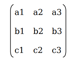
followed by translation by t1 in the x direction, t2 in the y direction and t3 in the z direction.
The trick is to replace each three-dimensional vector (x,y,z) with the four-dimensional vector (x,y,z,1), adding a "1" as the fourth coordinate. And instead of the 3-by-3 matrix, we use the 4-by-4 matrix:
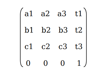
If the vector (x1,y1,z1,1) is multiplied by this 4-by-4 matrix, the result is precisely the vector (x2,y2,z2,1). That is, instead of applying an affine transformation to the 3D vector (x1,y1,z1), we can apply a linear transformation to the 4D vector (x1,y1,z1,1).
This might seem pointless to you, but nevertheless, that is what is done in OpenGL and other 3D computer graphics systems: An affine transformation is represented as a 4- by-4 matrix in which the bottom row is (0,0,0,1), and a three-dimensional vector is changed into a four dimensional vector by adding a 1 as the final coordinate.
The result is that all the affine transformations that are so important in computer graphics can be implemented as multiplication of vectors by matrices.
The identity transformation, which leaves vectors unchanged, corresponds to multiplication by the identity matrix, which has ones along its descending diagonal and zeros elsewhere.
The OpenGL function glLoadIdentity() sets the current matrix to be the 4-by-4 identity matrix.
An OpenGL transformation function, such as glTranslatef (tx,ty,tz), has the effect of multiplying the current matrix by the 4-by-4 matrix that represents the transformation.
Multiplication is on the right; that is, if M is the current matrix and T is the matrix that represents the transformation, then the current matrix will be set to the product matrix MT.
For the record, the following illustration shows the identity matrix and the matrices corresponding to various OpenGL transformation functions:
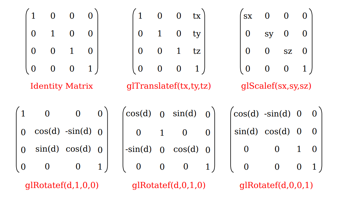
So if we want to translate the vector (10,10,10,1) of 10 units in the X direction, we get:

and we get a (20,10,10,1) homogeneous vector! Remember, the 1 means that it is a position, not a direction. So our transformation didn't change the fact that we were dealing with a position, which is good.
If we want to scale a vector (position or direction, it doesn't matter) by 2.0 in all directions:

and the w still didn't change. You may ask: what is the meaning of "scaling a direction"? Well, often, not much, so you usually don't do such a thing, but in some (rare) cases it can be handy.
There is one common transformation in computer graphics that is not an affine transformation: In the case of a perspective projection, the projection transformation is not affine.
In a perspective projection, an object will appear to get smaller as it moves farther away from the viewer, and that is a property that no affine transformation can express, since affine transforms preserve parallel lines and parallel lines will seem to converge in the distance in a perspective projection.
Surprisingly, we can still represent a perspective projection as a 4-by-4 matrix, provided we are willing to stretch our use of coordinates even further than we have already.
We have already represented 3D vectors by 4D vectors in which the fourth coordinate is 1. We now allow the fourth coordinate to be anything at all, except for requiring that at least one of the four coordinates is non-zero.
When the fourth coordinate, w, is non-zero, we consider the coordinates (x,y,z,w) to represent the three-dimensional vector (x/w,y/w,z/w). Note that this is consistent with our previous usage, since it considers (x,y,z,1) to represent (x,y,z), as before.
When the fourth coordinate is zero, there is no corresponding 3D vector, but it is possible to think of (x,y,z,0) as representing a 3D “point at infinity” in the direction of (x,y,z).
Coordinates (x,y,z,w) used in this way are referred to as homogeneous coordinates.
If we use homogeneous coordinates, then any 4-by-4 matrix can be used to transform threedimensional vectors, including matrices whose bottom row is not (0,0,0,1).
Among the transformations that can be represented in this way is the projection transformation for a perspective projection. And in fact, this is what OpenGL does internally.
It represents all three-dimensional points and vectors using homogeneous coordinates, and it represents all transformations as 4-by-4 matrices. You can even specify vertices using homogeneous coordinates.
For example, the command:
with a non-zero value for w, generates the 3D point (x/w,y/w,z/w). Fortunately, you will almost never have to deal with homogeneous coordinates directly (we'll talk more about that again later).
Nowadays 3D Computer graphics, or CG, are everywhere. From video games to medical applications.
The film industry is dominated by computers, and it's not just sci-fi and animation. While filming the Irishman, Martin Scorsese used computer effects to de-age actors Robert De Niro, Joe Pesci, and Al Pacino.
It's kind of crazy when you realize that the first feature film to incorporate computer generated imagery was Westworld, starring Yul Brynner and James Brolin. That was in 1973, more than 50 years ago!
Today, we have devices like the Meta Quest 3 and the Apple Vision Pro, which blend digital content with your physical space.
With all of this, it's clear that 3D computer graphics have become an integral component of our everyday lives. But, how are these computer graphics created?
The process usually begins with an artist or designer using 3D modeling software like Maya, Cinema4D, or Blender, just to name a few.
Artists usually start off with a simple shape like a box or a sphere and then use different tools to modify this geometry.
If not working with an artist (or being an artist yourself), there are various Graphics APIs.
Graphics APIs and pipelines are crucial in computer graphics. They enable developers to create visuals for video games, animations, or simulations. These systems are important for managing how images are drawn and displayed on the screen.
A Graphics API (Application Programming Interface) is a set of functions that allows programs to perform operations like drawing images and 3D surfaces.
Essentially, APIs provide a way for software to communicate with hardware. Graphics APIs focus specifically on creating and displaying visual content.
Every graphics program requires two key types of APIs:
There are two approaches for using graphics APIs:
Some languages, such as Java, have built-in graphics and user-interface APIs. This ensures portability. Where the code will work across different systems. Everything is standardized, making development simpler for beginners.
Direct3D and OpenGL are example of these types, where drawing commands are part of a software library. This approach is more powerful but can vary from system to system. It offers more control, portability can be an issue unless developers use an additional library to handle user interface differences.
Direct3D and OpenGL are the most popular and widely used Graphics APIs.
After the graphics APIs, let's look at the concept of graphics pipelines.
The following image shows a monkey head model created using the free and open source software Blender:
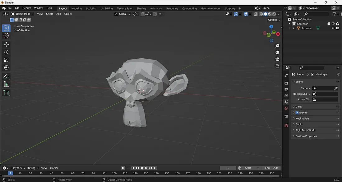
If we inspect the model closer, we can see that it's made up of a collection of points joined together with simple geometries. This structure of joined points is known as a Mesh.
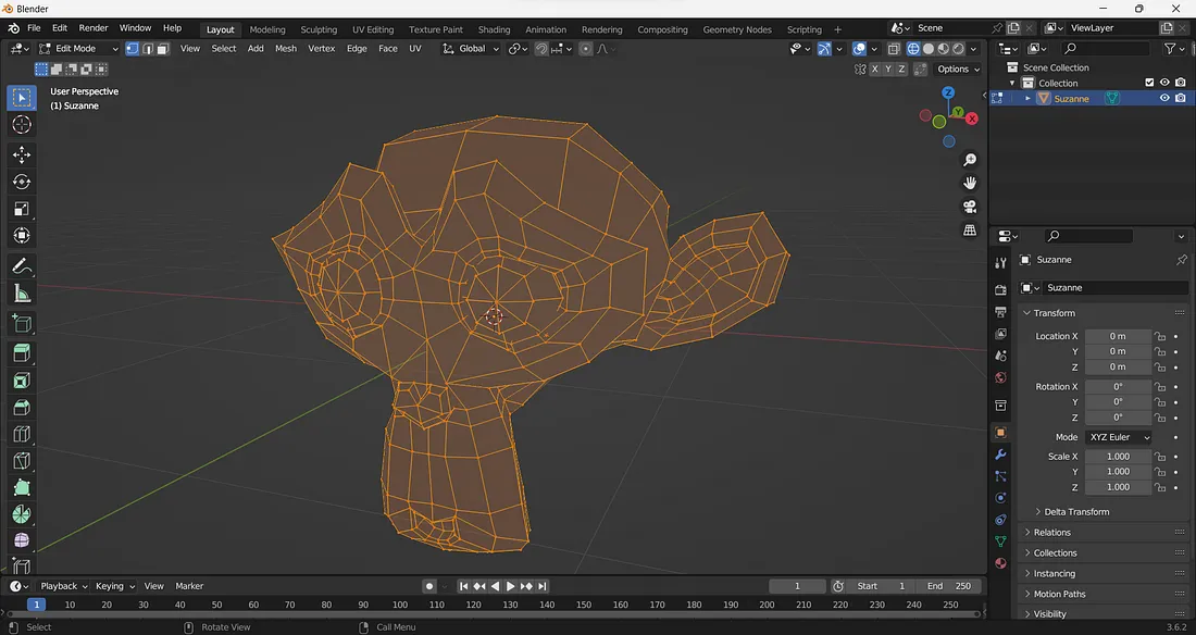
Each individual point is known as a vertex. A vertex is a point in space that has coordinates x, y, and z which determine its position in the 3D world.
So, meshes are made up of vertices and vertices are made up of coordinate values. But how do we go from three numerical values to something on the screen?
A graphics pipeline is a sequence of stages that transform data from a mathematical representation to something on a screen.
In essence, all 3D objects are just data. Data can live in a 3D space, however, our screen is not 3D. We need to take vertices in 3D space through a series of stages in order to transform them to a 2D space.
In other words, these are the process that computers follow to create 3D images and display them on a 2D screen. It is a series of steps that take the input, such as the geometry of 3D models, and turn it into pixels on the screen.
Let's start with the first stage: the Vertex Shader.
This is the first step where the positions of 3D points (vertices) are calculated. These vertices form the basic structure of 3D objects. For example, if we are rendering a car in a racing game, the position of each vertex of the car model is calculated in this stage
Imagine we have a simple cube. This cube geometry is defined as a list of 8 vertices.
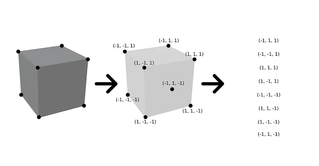
The vertex shader first transforms these vertices from a space where they are relative to their own origin, to a new space where everything is in relation to a camera's position and orientation.
Finally, we take vertices from a 3D coordinate system into a 2D plane by using perspective projection.
Projection creates the illusion of depth by scaling an object's coordinates based on their distance from the camera. This simulates how objects appear smaller as they move away from the viewer.
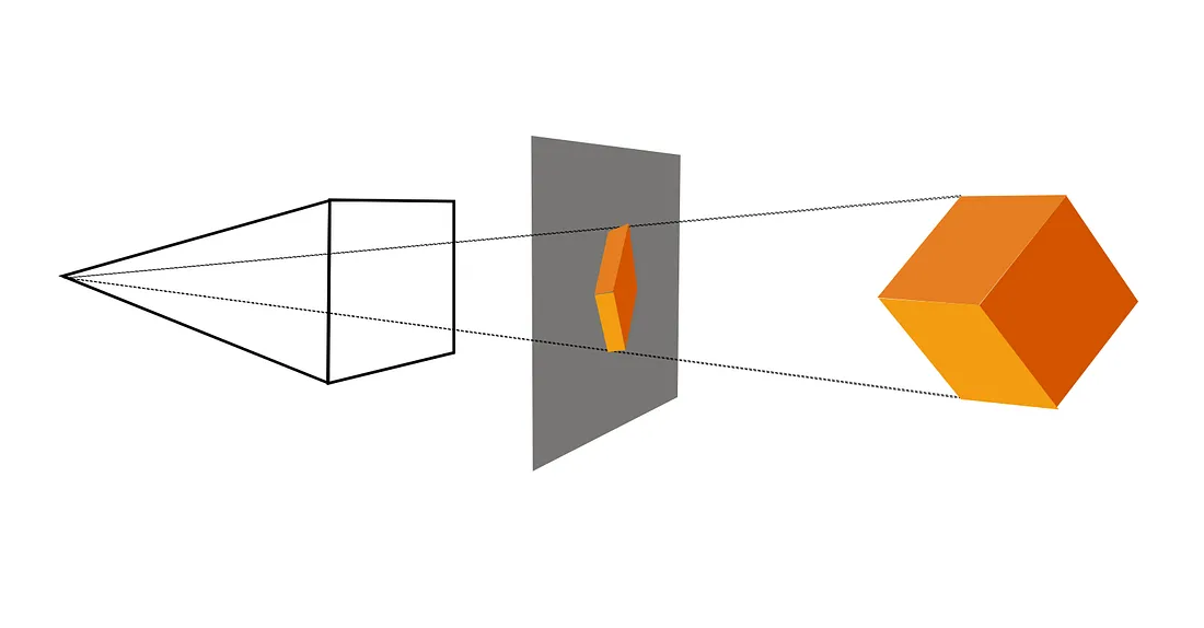
Now that our vertices have been transformed to a 2D space, it's time for the second stage: the primitive assembly.
Once vertices have been transformed, it's time for the primitive assembly.
In this stage, vertices are connected through geometric primitives. We can choose to use lines, points, or triangles.
Most modern graphics hardware are optimized to process triangles efficiently, that is why we usually choose them over lines and points.
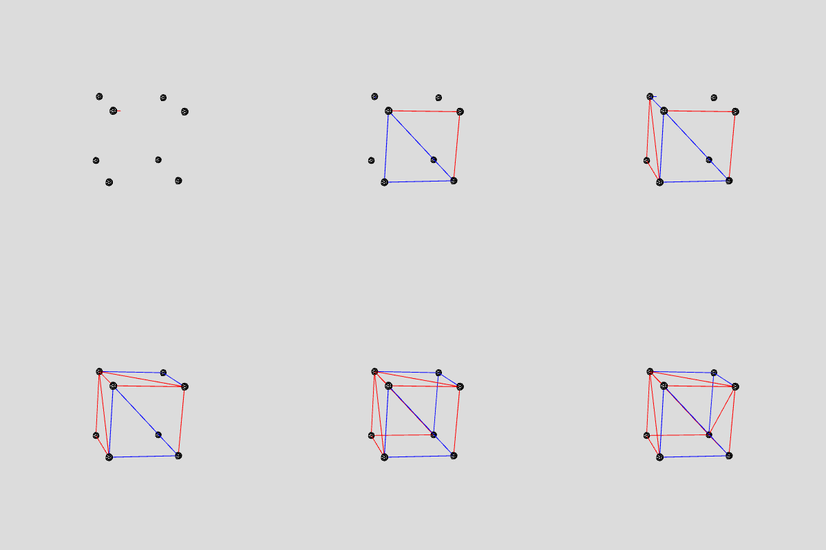
The primitive assembly lays the groundwork for the next step, which is rasterization.
The next important step is rasterization. This is where the 3D models are converted into pixels or fragments. These pixels represent the final image that will appear on the screen. For example, the 3D model of a tree in a game is converted into a collection of colored pixels that represent the tree on the screen.
We now have geometry made up of 3 dimensional vertices projected onto a 2D screen.
The rasterization step determines which pixels are inside the triangle. It breaks the shape into small fragments or pixels.
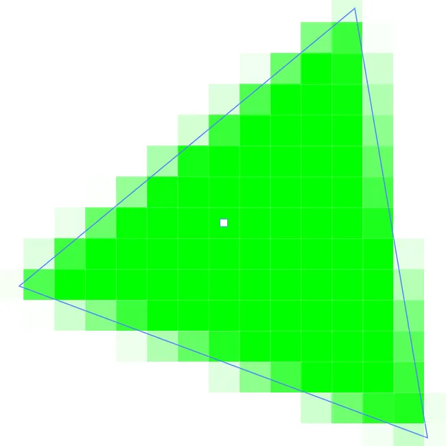
Rasterization not only determines which pixels are inside the shape, but also improves performance by discarding triangles which are not visible or occluded. This is known as Culling.
Culling determines which triangles are facing away from the camera, are outside of the camera's view, or simply hidden by another object.
In this case the triangle gets discarded and the computational load on the GPU (Graphical Processing Unit ) is reduced.
The next stage in the pipeline is known as the fragment shader.
After rasterization, the triangle is broken into pixel fragments. These individual pixel fragments are then processed by the fragment shader.
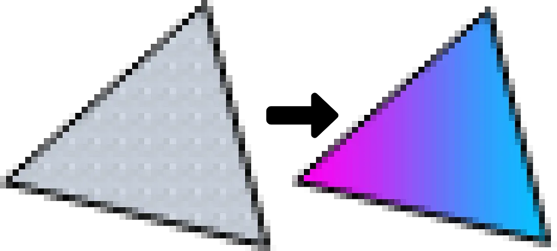
In this step we determine a color for each of the pixels that belong to the triangle. We do this by taking into account the material properties of the object, textures, and light sources in the scene.
With all of these information, we perform some calculations that determine the final color of the fragment.
Finally, all of the shaded fragments are copied to the framebuffer, which is basically the image displayed on the screen.
You can think of the framebuffer as a canvas where everything gets stored before being displayed on the screen.
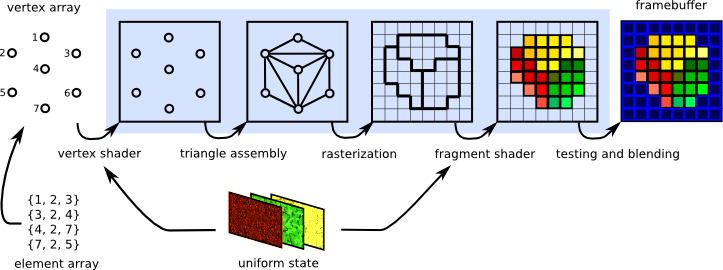
This is a general overview of a typical graphics pipeline. Note that there may be different pipelines, which have additional steps that we ignored.
Earlier versions of graphics libraries offered "fixed" pipeline. This means that the process had predefined stages and operations. Specifically, the vertex and fragment shaders. Developers had limited control over how these specific stages behaved.
With older pipelines, we would simply define the vertex data, material data, and lighting. Then, we would send this data to the GPU and we'd get a result. This was easier for beginners, but provided little room for modification and customization. For example, the lighting model used could not be changed.
In modern graphics libraries, "fixed" pipelines are deprecated in favor of "programmable" pipelines. Modern pipelines provide greater flexibility and control over the rendering process. However, you must provide the code for the vertex and fragment shader yourself. This means more control for the developer, but an additional layer of difficulty for beginners.
Shader programs are written in a C style language called GLSL (OpenGL Shading Language). Shader programs run on the GPU, which is different from how programs run on the CPU. The CPU executes tasks sequentially, while the GPU executes tasks in parallel.
The fact is that this extra layer is worth it! We can achieve great results with these new pipelines. There is also a thriving community of creative individuals that are constantly pushing this technology even further.
OpenGL is generally considered to be a cross-platform graphics API for high-performance 2D and 3D graphics rendering. In fact, OpenGL is not an API. It is a specification developed and maintained by the Khronos organization.
The specification strictly defines how each function should be executed and what their outputs should be. How each function is implemented internally is up to the developer.
It is widely used in video games, CAD, virtual reality, scientific visualization, and more.
WebGL (Web Graphics Library) is a JavaScript API for rendering interactive 2D and 3D graphics within any compatible web browser without the use of plug-ins.
It is based on OpenGL ES (a subset of OpenGL for embedded systems).
Major browser vendors Apple (Safari), Google (Chrome), Microsoft (Edge), and Mozilla (Firefox) are members of the WebGL Working Group.
Three.js is a popular JavaScript library that simplifies the creation and display of 3D graphics in a web browser using WebGL.
It supports VR and AR, offers cross-browser compatibility via WebGL, provides extensive tools for adding materials, textures, and animations, and allows for the integration of models from other 3D modeling software.
All modern browsers became more powerful and more accessible directly using JavaScript. They have adopted WebGL (Web Graphics Library) and as previously mentioned, WebGL is a Javascript API that allows you to render 2D and 3D graphics without the use of plugins. Trying to create 3D elements with WebGL would involve writing lots of code and can get fairly complex.
Three.js helps simplify the process and is essentially an abstracted layer on top of WebGL that makes it easier to use.
Three.js is an open-source, lightweight, cross-browser, general-purpose JavaScript library. Three.js uses WebGL behind the scenes, so you can use it to render Graphics on an HTML canvas element in the browser.
Since Three.js uses JavaScript, you can interact with other web page elements, add animations and interactions, and even create a game with some logic.
Three.js works with the HTML canvas element, the same thing that we used for 2D graphics. In almost all web browsers, in addition to its 2D Graphics API, a canvas also supports drawing in 3D using WebGL, which is used by three.js and which is about as different as it can be from the 2D API.
The following features make Three.js an excellent library to use:
With a couple of lines of JavaScript and simple logic, you can create anything, from highperformance interactive 3D models to photorealistic real-time scenes.
We'll start by adding the following to our HTML:
<script src="https://cdnjs.cloudflare.com/ajax/libs/three.js/r128/three.min.js"></script>Before you can use three.js, you need somewhere to display it.
To actually be able to display anything with three.js, we need three things:
const scene = new THREE.Scene();
const camera = new THREE.PerspectiveCamera(75, 500 / 400, 0.1, 1000);
const renderer = new THREE.WebGLRenderer();
renderer.setSize(500, 400);
document.body.appendChild(renderer.domElement);
Now, let's break down each of these components.
A scene is the container object that includes everything we will be rendering, such as geometries, lights, and cameras. In a sense, it's much like a stage where you place all the elements you want to display.
We create an instance of the scene object using the constructor with no parameters: THREE.Scene()
The function scene.add(item) can be used to add cameras, lights, and graphical objects to the scene. It is probably the only scene function that you will need to call. The function scene.remove(item), which removes an item from the scene, is also occasionally useful.
Next, we create a camera which will be how we view the scene.
The camera displays the objects in the scene, with varying points of view depending on which type of camera is used.
The Three.js library provides two main cameras: Orthographic and Perspective.
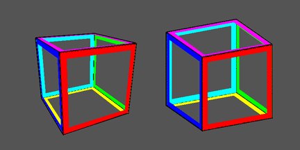
In a perspective view (left), edges that are farther away appear shorter.
In an Orthographic view (right), far-away edges are the same size as nearby ones.
The constructors specify the projection, using parameters that are familiar from OpenGL:
or:
Since the PerspectiveCamera is more common, let's go over its four attributes:
The first parameter it takes is the field of view (FOV), the maximum area of the scene that can be viewed. To help visualize, picture a cone coming out of a camera lens, and the flat end of the cone is the space the camera can see. This value is measured in degrees.
Next is the aspect ratio, which is the proportion of the width to the height of the element.
You almost always want to use the width of the element divided by the height, or you'll get the same result as when you play old movies on a widescreen TV - the image looks squished.
The near and far attributes are the minimum and maximum distance from the camera at which the camera will render scene objects. Anything beyond these values, either too close or too far from the camera, will not be rendered.
Finally, once the camera is set up, you need to add it to the scene.
Remember to append everything to your container to make it show on your scene.
Keep in mind that by default, when you add something to the scene, it will be placed in the center at the XYZ coordinates 0, 0, 0 respectively. So if you have trouble seeing anything you have added render in the scene, chances are you might need to position your camera further out of view.
For example, setting the camera's Z coordinate to 5:
camera.position.z = 5;The last step is to render the scene. The renderer is what compiles it all together and draws the scene.
We need to create the renderer instance, we will use WebGLRenderer() but three.js comes with others as well, often used as fallbacks for users with older browsers/who don't have WebGL support.
We also need to set the size at which we want it to render our app.
In the following examples we will use a width of 500 and a height of 400, though it is common to use the width and height of the browser window (window.innerWidth, window.innerHeight) as well.
Lastly, we add the renderer element to our HTML document. This is a canvas element the renderer uses to display the scene to us.
A renderer is an instance of the class THREE.WebGLRenderer. Its constructor has one parameter, which is a JavaScript object containing settings that affect the renderer.
All together our code should look something like this:
const scene = new THREE.Scene(); //Creates a new instance of the Scene class.
const camera = new THREE.PerspectiveCamera(50, 500 / 400, 0.1, 1000); //Creates a new instance of the PerspectiveCamera class with a field of view of 50 degrees, an aspect ratio of 500/400, a near clipping plane of 0.1, and a far clipping plane of 1000.
camera.position.z = 5; //Moves the camera 5 units away from the center of the scene.
const renderer = new THREE.WebGLRenderer(); //Creates a new instance of the WebGLRenderer class.
renderer.setSize(500, 400); //Sets the size of the renderer to 500px by 400px.
document.body.appendChild(renderer.domElement); //Appends the renderer's canvas element to the document body to display the rendered scene.
However, just defining an instance of the renderer is not enough to see the results of our code yet, because we have not actually rendered anything as of yet.
To achieve this, we will need to create a render or animate loop, like this:
function animate() {
    requestAnimationFrame(animate);
    renderer.render(scene, camera);
}

animate();
We have now created a loop named animate() that causes the renderer to draw the scene every time the screen is refreshed (on a typical screen, this is about 60 times per second), and called it immediately after.
Using requestAnimationFrame() has a number of advantages, such as pausing when the user navigates to another browser tab, saving processing power and battery life.
Now we've successfully set up out scene! Now for the fun part, we can start creating the shapes that we would like to add to our scene.
Much like how we need three elements to set a scene, objects require three elements:
Let's start with the first element, the geometry.
The geometry defines the shape of the objects we draw in Three.js.
It is made up of a collection of vertices and faces which combine three vertices into a triangle face.
There are two main types of geometries in Three.js:
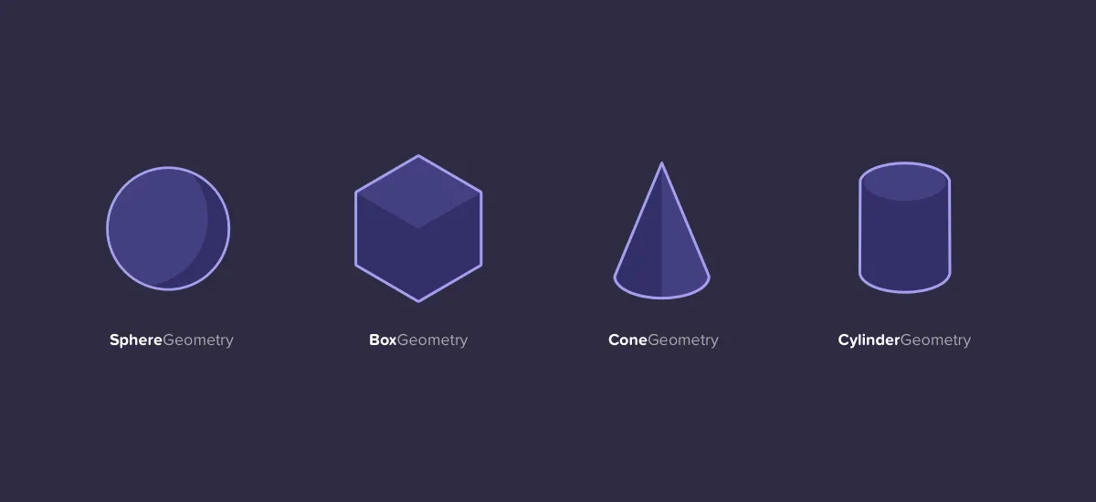
Here are some constructors, listing all parameters (but keep in mind that most of the parameters are optional):
The class BoxGeometry represents the geometry of a rectangular box centered at the origin.
Its constructor has three parameters to give the size of the box in each direction; their default value is one.
The last three parameters give the number of subdivisions in each direction, with a default of one; values greater than one will cause the faces of the box to be subdivided into smaller triangles.
The class PlaneGeometry represents the geometry of a rectangle lying in the xy-plane, centered at the origin. Its parameters are similar to those for a cube.
A RingGeometry represents an annulus, that is, a disk with a smaller disk removed from its center. The ring lies in the xy-plane, with its center at the origin. You should always specify the inner and outer radii of the ring.
The constructor for ConeGeometry has exactly the same form and effect as the constructor for CylinderGeometry, with the radiusTop set to zero. That is, it constructs a cone with axis along the y-axis and centered at the origin
For SphereGeometry, all parameters are optional.
The constructor creates a sphere centered at the origin, with axis along the y-axis.
The first parameter, which gives the radius of the sphere, has a default of one.
The next two parameters give the numbers of slices and stacks, with default values 32 and 16.
The last four parameters allow you to make a piece of a sphere; the default values give a complete sphere. The four parameters are angles measured in radians. phiStart and phiLength are measured in angles around the equator and give the extent in longitude of the spherical shell that is generated.
For example:
creates the geometry for the "western hemisphere" of a sphere.
The last two parameters are angles measured along a line of latitude from the north pole of the sphere to the south pole.
For example, to get the sphere's "northern hemisphere":
For TorusGeometry, the constructor creates a torus lying in the xy-plane, centered at the origin, with the z -axis passing through its hole.
The parameter radius is the distance from the center of the torus to the center of the torus's tube, while tube is the radius of the tube. The next two parameters give the number of subdivisions in each direction.
The last parameter, arc, allows you to make just part of a torus. It is an angle between 0 and 2*Math.PI, measured along the circle at the center of the tube.
There are also geometry classes representing the regular polyhedra: THREE.TetrahedronGeometry, THREE.OctahedronGeometry, THREE.DodecahedronGeometry, and THREE.IcosahedronGeometry. (For a cube use a BoxGeometry.)
The constructors for these four classes take two parameters. The first specifies the size of the polyhedron, with a default of 1. The size is given as the radius of the sphere that contains the polyhedron.
The second parameter is an integer called detail. The default value, 0, gives the actual regular polyhedron. Larger values add detail by adding additional faces.
As the detail increases, the polyhedron becomes a better approximation for a sphere. This is easier to understand with an illustration:

The image shows four mesh objects that use icosahedral geometries with detail parameter equal to 0, 1, 2, and 3.
Materials describe the appearance of objects.
They are defined in a (mostly) renderer-independent way, so you don't have to rewrite materials if you decide to use a different renderer.
There are different types of materials:
The next materials however, DO require lights in order to be seen:
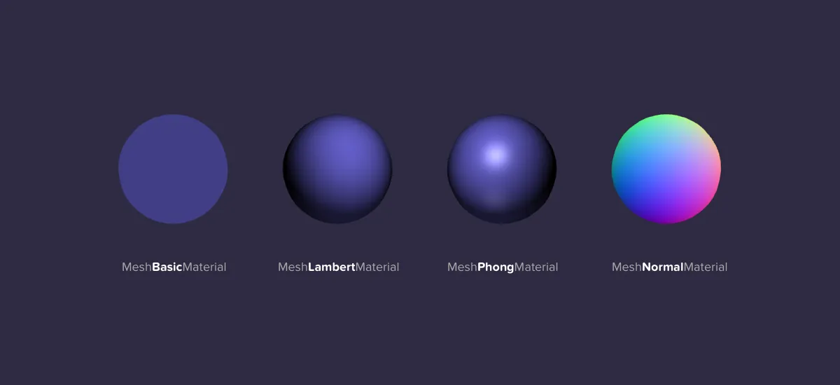
A Mesh is a class representing triangular polygon mesh based objects.
A Mesh pairs a Geometry and a Material in order to draw/create an object.
Both Material objects and Geometry objects can be used by multiple Mesh objects.
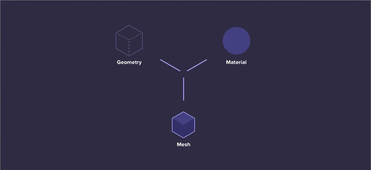
Now that we have our scene, camera, renderer, geometry, material, and mesh, we can start creating our objects.
Although we'll mostly focus on 3D objects in Three.js, let's start with a simple 2D triangle.
We can create this triangle using BufferGeometry:
var size = 2;

function createTriGeometry(size) {
    const triGeom = new THREE.BufferGeometry();

    // Define the vertices of the triangle
    const vertices = new Float32Array([
        0, 0, 0, // Vertex 1
        size, 0, 0, // Vertex 2
        0, size, 0  // Vertex 3
    ]);

    // Set the vertices as attribute
    triGeom.setAttribute('position', new THREE.BufferAttribute(vertices, 3));

    // Define the indices for the single triangle face
    const indices = new Uint16Array([
        0, 1, 2 // A single face made up of the three vertices
    ]);

    // Set the indices
    triGeom.setIndex(new THREE.BufferAttribute(indices, 1));

    return triGeom;
}

// Create the triangle geometry
var triGeom1 = createTriGeometry(size);

// Define the material for the triangle
var triMaterial = new THREE.MeshBasicMaterial({
    color: new THREE.Color("red"),
    side: THREE.DoubleSide // Render both sides of the triangle
});

// Create the mesh with geometry and material
var triMesh1 = new THREE.Mesh(triGeom1, triMaterial);

// Add triangle to the scene
scene.add(triMesh1);
In this code we:
Now, when we run the code, we should see a red triangle rendered in the scene.
Let's adjust the background color:
scene.background = new THREE.Color("blue");Now our red triangle should be displayed on a blue background.
Let's create a simple square using BufferGeometry:
const geometry = new THREE.BufferGeometry();
// create a simple square shape. We duplicate the top left and bottom right
// vertices because each vertex needs to appear once per triangle.
const vertices = new Float32Array( [
	-1.0, -1.0,  1.0, // v0
	 1.0, -1.0,  1.0, // v1
	 1.0,  1.0,  1.0, // v2

	 1.0,  1.0,  1.0, // v3
	-1.0,  1.0,  1.0, // v4
	-1.0, -1.0,  1.0  // v5
]);

geometry.setAttribute('position', new THREE.BufferAttribute(vertices, 3));
const material = new THREE.MeshBasicMaterial({ color: 0x00ff00 });
const cube = new THREE.Mesh(geometry, material);

scene.add(cube);
Now, when you run the code, you should see a green square (cube) rendered in the scene.
Here we create a BufferGeometry object and pass in an array of vertices that define the square's shape.
Next, we create a MeshBasicMaterial object and pass in a color parameter to give the square a green color.
Finally, we create a Mesh object by passing in the geometry and material objects, and add it to the scene.
Notice this only makes a 2D square out of two triangles, but we can make a 3D cube by adding more vertices and faces.
// Define vertices for a cube
const vertices = new Float32Array([
    // Front face
    -1.0, -1.0,  1.0,
     1.0, -1.0,  1.0,
     1.0,  1.0,  1.0,
     1.0,  1.0,  1.0,
    -1.0,  1.0,  1.0,
    -1.0, -1.0,  1.0,

    // Back face
    -1.0, -1.0, -1.0,
    -1.0,  1.0, -1.0,
     1.0,  1.0, -1.0,
     1.0,  1.0, -1.0,
     1.0, -1.0, -1.0,
    -1.0, -1.0, -1.0,

    // Top face
    -1.0,  1.0, -1.0,
    -1.0,  1.0,  1.0,
     1.0,  1.0,  1.0,
     1.0,  1.0,  1.0,
     1.0,  1.0, -1.0,
    -1.0,  1.0, -1.0,

    // Bottom face
    -1.0, -1.0, -1.0,
     1.0, -1.0, -1.0,
     1.0, -1.0,  1.0,
     1.0, -1.0,  1.0,
    -1.0, -1.0,  1.0,
    -1.0, -1.0, -1.0,

    // Right face
     1.0, -1.0, -1.0,
     1.0,  1.0, -1.0,
     1.0,  1.0,  1.0,
     1.0,  1.0,  1.0,
     1.0, -1.0,  1.0,
     1.0, -1.0, -1.0,

    // Left face
    -1.0, -1.0, -1.0,
    -1.0, -1.0,  1.0,
    -1.0,  1.0,  1.0,
    -1.0,  1.0,  1.0,
    -1.0,  1.0, -1.0,
    -1.0, -1.0, -1.0
]);

// Create geometry and material
const geometry = new THREE.BufferGeometry();
geometry.setAttribute('position', new THREE.BufferAttribute(vertices, 3));

const material = new THREE.MeshBasicMaterial({ color: 0x00ff00 });

// Create cube mesh
const cube = new THREE.Mesh(geometry, material);
scene.add(cube);
Now we should be able to see a cube since we have defined the vertices of each of the six faces.
Understanding this is important, although not entirely necessary since we are merely creating a cube. We can simplify this process by using BoxGeometry() instead of BufferGeometry().
BoxGeometry is a geometry class for a rectangular cuboid with a given 'width', 'height', and 'depth'. How can we obtain the same scaled 2D shape using BoxGeometry()?
To create a cube without declaring all vertices, we use BoxGeometry. This is an object that contains all the points (vertices) and fill (faces) of the cube.
Let's set the width, height, and depth to 2 respectively, because our previous square had a width, height, and depth of 2 as well! (if we do not set it at all, the w/h/d defaults to 1, try changing the values! How does this change the object?)
const geometry = new THREE.BoxGeometry(2, 2, 2);Notice how since our structure is a simple cube we have no need for a group of vertices since the same result can be obtained in one line of code!
We'll definitely use vertices for more irregular polygons but for now, BoxGeometry works just fine!
Let's add X and Y-axis rotation to our cube. We can do this simply by adding the following to animate():
//Now to make it more interesting and dimensional, let's add a rotation animation
cube.rotation.x += 0.01;
cube.rotation.y += 0.01;
We can increase/decrease the speed of rotation by changing the values of cube.rotation.x and cube.rotation.y
Now, when you run the code, you should see the cube rotating on both the X and Y axes.
Let's make a multi-colored cube:
We can achieve this using an array of materials.
const materials = [
    new THREE.MeshBasicMaterial({ color: "green" }),
    new THREE.MeshBasicMaterial({ color: "blue" }),
    new THREE.MeshBasicMaterial({ color: "red" }),
    new THREE.MeshBasicMaterial({ color: "yellow" }),
    new THREE.MeshBasicMaterial({ color: "orange" }),
    new THREE.MeshBasicMaterial({ color: "purple" })
];
Now, when we run the code, we should see a cube with different colored faces.
Let's revert back to a singularly colored cube.
We can also change our cube to simply display the wireframe of our geometry by modifying our material:
const material = new THREE.MeshBasicMaterial({ color: "green", wireframe: true });Now let's change the material of our cube to MeshNormalMaterial:
const material = new THREE.MeshNormalMaterial();Now, let's look at a wireframe to our cube:
const wireframe = new THREE.WireframeGeometry(geometry);
const line = new THREE.LineSegments(wireframe);
line.material.depthTest = false;
line.material.opacity = 1;
line.material.transparent = true;
scene.add(line);
This is good if we want a wireframe in addition to our solid object.
If we want it to rotate remember to update the rotations as well.
A helpful tool to implement when creating your projects is dat.GUI.
In Javascript, dat.GUI is a lightweight graphics controller API. It allows the user to manipulate variables easily and activate functions inside the application by providing a graphical controller interface.
This API is frequently used in Three.js for making changes to a scene without having to refer directly to the code.
It will be displayed as a small box in the corner of your screen and you can play around with the parameters and see the newly applied changes happen live.
It's a great tool to use when you want to experiment with different values and see how they affect your project.
Here's how we can add dat.GUI to our project:
First, we need to ensure that we have access to dat.GUI by adding this line to our HTML:
<script src="https://cdnjs.cloudflare.com/ajax/libs/dat-gui/0.7.6/dat.gui.min.js"></script>Next, we can add the following code to our JavaScript:
const gui = new dat.GUI();
gui.add(cube.rotation, 'x', 0, Math.PI * 2);
gui.add(cube.rotation, 'y', 0, Math.PI * 2);
Now, when we run the code, we should see the dat.GUI box in the corner of our screen.
By changing the values of the sliders, we can adjust the rotation of the cube on the X and Y axes.
And that's it! We've successfully added dat.GUI to our project.
Let's add a color changer to our dat.GUI as well:
// Add GUI for controls
const gui = new dat.GUI();
const cubeFolder = gui.addFolder('Cube Properties');

const cubeParams = {
    color: `#${material.color.getHexString()}`,
    rotationX: 0,  // New parameter for X rotation angle
    rotationY: 0   // New parameter for Y rotation angle
};

// Color control
cubeFolder.addColor(cubeParams, 'color').onChange((value) => {
    cube.material.color.set(value);
});

// X rotation control
cubeFolder.add(cubeParams, 'rotationX', -Math.PI, Math.PI).name('Rotation X').onChange((value) => {
    cube.rotation.x = value;
});

// Y rotation control
cubeFolder.add(cubeParams, 'rotationY', -Math.PI, Math.PI).name('Rotation Y').onChange((value) => {
    cube.rotation.y = value;
});

cubeFolder.open();Now that we've created a cube, let's create a sphere using SphereGeometry().
const scene = new THREE.Scene();
const camera = new THREE.PerspectiveCamera(50, 500 / 400, 0.1, 1000);
const renderer = new THREE.WebGLRenderer();
renderer.setSize(500, 400);
document.body.appendChild(renderer.domElement);

camera.position.z = 7;

//sphere:
const material = new THREE.MeshBasicMaterial({
    color: "orange"
});
const geometry = new THREE.SphereGeometry(2, 50, 50); //radius, widthSegments, heightSegments
const sphere = new THREE.Mesh(geometry, material);
scene.add(sphere);

function animate() {
    requestAnimationFrame(animate);
    renderer.render(scene, camera);
}

animate();
We should see a basic Three.js code snippet creating an orange sphere on canvas. Nothing fancy. The sphere is made from a basic material which does not respond to light, therefore we can see the model as is.
We can turn this sphere into a wireframe like we did before, by using WireframeGeometry or we can simply add another specification to our original material.
Let's add a wireframe to our sphere:
const material = new THREE.MeshBasicMaterial({
    color: "orange",
    wireframe: true //sets the wireframe
});
Now, when we run the code, we should see an orange wireframe sphere rendered in the scene.
Let's rotate it by adding the following lines to our animate function:
sphere.rotation.x += 0.01;
sphere.rotation.y += 0.01;
Now, when you run the code, you should see the sphere rotating on both the X and Y axes.
Let's add dat.GUI to our sphere that only includes a checkbox that helps us toggle from our original orange color to a blue wireframe:
const gui = new dat.GUI();
const sphereFolder = gui.addFolder('Sphere Properties');

const sphereParams = {
    blue: false
};

// Wireframe color control
sphereFolder.add(sphereParams, 'blue').name('blue wireframe').onChange((value) => {
    if (value) {
        sphere.material.color.set('blue');
    } else {
        sphere.material.color.set('orange');
    }
});

sphereFolder.open(); //to start with the folder open
Now when you run the code, you should see a checkbox in the dat.GUI box that allows you to toggle between the original orange color and a blue wireframe for the sphere.
So we've seen objects with simple materials like MeshBasicMaterial and MeshNormalMaterial that did not need lighting, however to render a scene realistically we need to add lights.
There are several types of lights in Three.js:
AmbientLight does not point or direct light toward a direction, so it cannot cast shadows, contributes just a little light/brightness to the scene.
The first parameter is the color and the second parameter is the intensity:
// Ambient light
const ambientLight = new THREE.AmbientLight("green", 1); //color, intensity
scene.add(ambientLight);
Let's look at an example: Ambient Light Example
Notice how if we remove the light from our scene we cannot see the cube anymore. That is because it is made out of MeshPhongMaterial, we'll talk more about that a bit later with shading.
Just know that MeshPhongMaterial is a material that responds to lights and adds a metallic luster to the surface, reflecting light with more intensity. It computes lighting at every pixel.
If all you have is an AmbientLight, you'll have the same effect as for a MeshBasicMaterial because all faces of the geometries will be lit equally.
Like ambient light, hemisphere light has no position or direction. But unlike ambient light it has two colors.
This is to provide a bit more realism than a globally applied ambient light.
// Hemisphere light
const hemisphereLight = new THREE.HemisphereLight("blue", "green", 1); //skyColor, groundColor, intensity
scene.add(hemisphereLight);
Let's look at an example: Hemisphere Light Example
Notice how the cube is lit from the top with a blue light and from the bottom with a green light.
Direcional lights resemble the Sun. They're a distant powerful light source pointing in one direction.
They are positioned infinitely far away and emit light in a specific direction.
They have a color and intensity.
Directional lights are useful for simulating sunlight in a scene.
// Directional light
const directionalLight = new THREE.DirectionalLight("white", 1); //color, intensity
directionalLight.position.set(0, 1, 0); //x, y, z
scene.add(directionalLight);
Let's look at an example: Directional Light Example
Notice how the cube is lit from the top right corner. This is because the directional light is positioned at (0, 1, 0).
Let's add a second directional light to our scene:
// Directional light 2
const directionalLight2 = new THREE.DirectionalLight("red", 1); //color, intensity
directionalLight2.position.set(0, -1, 0); //x, y, z
scene.add(directionalLight2);
Now how does the cube look?
Point lights are like light bulbs in your scene.
They are positioned at a specific location and radiate light outwards in all directions from that postion. They have a color and intensity.
Point lights allow you to set the distance from the light at which point it's intensity is zero. You can also set the decay which is the amount the light dims along the distance.
// Point light
const pointLight = new THREE.PointLight("white", 1); //color, intensity
pointLight.position.set(5, 5, 5); //x, y, z
scene.add(pointLight);
Let's look at an example: Point Light Example
Notice how the cube is lit from the top right corner. This is because the point light is positioned at (5, 5, 5).
Let's add a second point light to our scene:
// Point light 2
const pointLight2 = new THREE.PointLight("blue", 1); //color, intensity
pointLight2.position.set(-5, -5, -5); //x, y, z
scene.add(pointLight2);Spotlights are just that, spotlights.
They are lights that point in one direction radiating out in a cone shape.
We can pass an angle to the light as a parameter which is the maximum angle of the light cone in radians.
Penumbra affects the intensity or softness of outer shadow or light fall-off as it fades to darkness.
Because spotlights have a direction they suffer from the same rotation behavior as directional lights, requiring them to point to a target object's position.
// Spot light
const spotLight = new THREE.SpotLight("white", 1); //color, intensity
spotLight.position.set(5, 5, 5); //x, y, z this is the position of the light
spotLight.target.position.set(0, 0, 0); //x, y, z this is the direction the light is pointing
scene.add(spotLight);
scene.add(spotLight.target);
Let's look at an example: Spot Light Example
Notice how the cube is lit from the top right corner. This is because the spot light is positioned at (5, 5, 5).
Let's add a second spot light to our scene:
// Spot light 2
const spotLight2 = new THREE.SpotLight("green", 1); //color, intensity
spotLight2.position.set(-5, -5, -5); //x, y, z this is the position of the light
spotLight2.target.position.set(0, 0, 0); //x, y, z this is the direction the light is pointing
scene.add(spotLight2);
scene.add(spotLight2.target);As previously mentioned, MeshPhongMaterial is a material for shiny surfaces with specular highlights.
Shading is calculated using a Phong shading model. The Phong shading model calculates shading per pixel (i.e. in the fragment shader, AKA pixel shader) which gives more accurate results/displays more realistic highlights.
The Phong model is made up of three distinct components:

And uses four vectors:
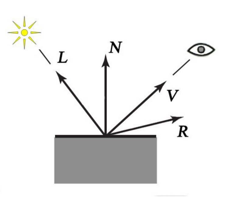
The following equation breaks it down:

The first part of the equation computes the diffuse light: shows the direction of the light and can show depth in an object.
The second part of the equation computes the specular highlight: for shiny objects and it reflects the bright spot on the surface. And the shininess coefficient α
The third part of the equation computes the ambient light: the background light for the object.
In summary:
There is also a Blinn-Phong shading model which is a modification of the Phong shading model.
Blinn-Phong, also known as the modified Phong model, uses the same equation, but measures the angle between the surface normal and the halfway vector instead of finding the angle between the view vector and the reflection vector.

where:

Although the material is called Phong it actually uses the Blinn-Phong reflection model rather than a pure Phong Reflection model.
Let's create a new material to see this in action:
const material = new THREE.MeshPhongMaterial({
   color: "red", // color to use for light, default is white
   shininess : 60, // shininess default is 30
   specular: "blue" // color of the specular highlight, default is white
});
Let's add some point lights so we can actually see the cube:
//Create point light and add to scene
const pointLight = new THREE.PointLight("white", 1); //color, intensity
pointLight.position.set(50, 50, 50); //x, y, z
scene.add(pointLight);


// Point light 2
const pointLight2 = new THREE.PointLight("white", 1); //color, intensity
pointLight2.position.set(-50, -50, -50); //x, y, z
scene.add(pointLight2);
Now, when you run the code, you should see a red cube with a blue specular highlight rendered in the scene.
So far, we made the cube rotate automatically as it is rendered. This time let's try to control its rotation with user interaction.
To do this, we will comment out the rotational behavior and write our own.
We will use the arrow keys to control how to cube rotates. How do we make sure that the program is aware when we press a specific key and react accordingly?
As we saw a bit in 2D graphics, we will have to add anevent listener to attach an event handler to a specified element. In this case, we do not need to specify a particular element so we can attach an event handler to the document directly.
This is proper syntax for creating an event listener for the arrow keys:
// Add listener for keyboard
document.addEventListener('keydown', keyPressed);

//behavior for directional keys
function keyPressed(e){
  switch(e.key) {
    case "ArrowLeft": //left arrow
      //move left on the y-axis
    	cube.rotation.y -= 0.1;
    	break;
  	case "ArrowUp": //up arrow
      //move up on the x-axis
    	cube.rotation.x -= 0.1;
    	break;
    case "ArrowRight": //right arrow
      //move right on the y-axis
    	cube.rotation.y += 0.1;
    	break;
    case "ArrowDown": //down arrow
      //move down on the x-axis
    	cube.rotation.x += 0.1;
    	break;
  }
}
Now, when we run the code, we should be able to control the rotation of the cube using the arrow keys.
We've successfully added basic interactivity to our project.
Another way to add interactivity to your Three.js project is by using OrbitControls.
OrbitControls is a utility that allows you to control the camera in your scene using the mouse.
It allows you to rotate, zoom, and pan the camera around the scene.
Here's how you can add OrbitControls to your project:
First, you need to include the OrbitControls script in your HTML:
<script src="https://cdn.jsdelivr.net/npm/three@0.132.2/examples/js/controls/OrbitControls.js"></script>Next, you can add the following code to your JavaScript:
const controls = new THREE.OrbitControls(camera, renderer.domElement);
controls.update();
Now, when you run the code, you should be able to control the camera in your scene using the mouse.
And that's it! We've successfully added both mouse and keyboard interaction.
Shadows are an important part of creating a realistic 3D scene.
The light that is coming from a specific direction can cast shadows. First, we should make the scene ready for casting shadows.
We should first tell the renderer that we want to enable shadows. Casting shadows is an expensive operation. WebGLRenderer only supports this functionality.
It uses Shadow mapping, a technique specific to WebGL, performed directly on the GPU.
renderer.shadowMapEnabled = true;The above line of code tells the renderer to cast shadows in the scene.
Note - Three.js, by default, uses shadow maps. Shadow map works for light that casts shadows. The scene renders all objects marked to cast shadows from the point of view of the light.
There are two types of shadows in Three.js:
Shadow Mapping: This is the most common technique used to create shadows in 3D graphics. It works by rendering the scene from the perspective of the light source and storing the depth values of the scene in a texture called the shadow map. When rendering the scene from the camera's perspective, the depth values of the scene are compared to the depth values in the shadow map to determine if a pixel is in shadow or not.Shadow mapping is the method of choice for creating shadows in high-end rendering for motion pictures and television. However, it has been problematic to use shadow mapping in real-time applications, such as video games, because of aliasing problems in the form of magnified jaggies.
Shadow mapping involves projecting a shadow map on geometry and comparing the shadow map values with the light-view depth at each pixel. If the projection causes the shadow map to be magnified, aliasing in the form of large, unsightly jaggies will appear at shadow borders.
Aliasing can usually be reduced by using higher-resolution shadow maps and increasing the shadow map resolution, using techniques such as perspective shadow maps (Stamminger and Drettakis 2002).
However, using perspective shadow-mapping techniques and increasing shadow map resolution does not work when the light is traveling nearly parallel to the shadowed surface, because the magnification approaches infinity.
High-end rendering software solves the aliasing problem by using a technique called percentage-closer filtering.
PCF (Percentage-Closer Filtering): This is a technique used to smooth out the edges of shadows by taking multiple samples around each pixel and averaging the results. This helps to reduce the jagged appearance of shadows and create a more realistic effect.
Unlike normal textures, shadow map textures cannot be prefiltered to remove aliasing. Instead, multiple shadow map comparisons are made per pixel and averaged together.
This technique is called percentage-closer filtering (PCF) because it calculates the percentage of the surface that is closer to the light and, therefore, not in shadow.
The original PCF algorithm, described in Reeves et al. 1987, called for mapping the region to be shaded into shadow map space and sampling that region stochastically (that is, randomly).
The algorithm was first implemented using the REYES rendering engine, so the region to be shaded meant a four-sided micropolygon. The figure below shows an example of that implementation.
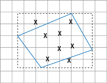
However, this algorithm advances over time.
For instance, NVIDIA GPUs have changed the PCF algorithm slightly to make it easy and efficient to apply. Instead of calculating the region to be shaded in shadow map space, they simply use a 4x4-texel sample region everywhere.
This region is large enough to significantly reduce aliasing, but not so large as to require huge numbers of samples or stochastic sampling techniques to achieve good results. Note that the sampling region is not aligned to texel boundaries.
PCF is a simple and effective way to reduce aliasing in shadow maps. It is not perfect, but it is a good compromise between quality and performance.
Since we are on the topic of antialiasing, we should also make sure that our scene is rendered with it enabled.
renderer.antialias = true;By doing this we can reduce the jagged edges of our objects.
Let's create a scene with shadows:
First, we need to enable shadows in our renderer:
renderer.shadowMap.enabled = true;Next, we need to enable shadows for each light that we want to cast shadows:
// Enable shadows for directional light
const light = new THREE.DirectionalLight(0xffffff, 1);
light.position.set(5, 5, 5); // Position the light
light.castShadow = true; // Enable shadow casting for the light
scene.add(light);
We should configure objects to cast shadows. We can inform Three.js which objects can cast shadows and which objects can receive shadows.
object1.castShadow = true;
object2.recieveShadow = true;
Let's create a simple cube that casts a shadow on a floor:
// Create a cube that casts a shadow
const cubeGeometry = new THREE.BoxGeometry(2, 2, 2);
const cubeMaterial = new THREE.MeshStandardMaterial({ color: "red" });
const cube = new THREE.Mesh(cubeGeometry, cubeMaterial);
cube.position.set(0, -1, 0);
cube.castShadow = true;
scene.add(cube);

// Create a floor that receives shadows
const floorGeometry = new THREE.PlaneGeometry(20, 20);
const floorMaterial = new THREE.MeshStandardMaterial({ color: "gray" });
const floor = new THREE.Mesh(floorGeometry, floorMaterial);
floor.rotation.x = -Math.PI / 2;
floor.position.y = -2;
floor.receiveShadow = true;

scene.add(floor);
Let's see how the shadow looks with a BasicShadowMap:
renderer.shadowMapType = THREE.BasicShadowMap;If our shadow looks a bit blocky around its edges, it means the shadow map is too small.
To increase the shadow map size, we can define shadowMapHeight and shadowMapWidth properties for the light.
Alternatively, we can also try to change the shadowMapType property of WebGLRenderer. We can set this to THREE.BasicShadowMap, THREE.PCFShadowMap, or THREE.PCFSoftShadowMap.
Now let's try to antialias the shadow:
// to antialias the shadow
renderer.shadowMapType = THREE.PCFSoftShadowMap;
// or
directionalLight.shadowMapWidth = 2048;
directionalLight.shadowMapHeight = 2048;Now that we've learned how to add shadows to our scene, add another object that casts a shadow on the floor:
Let's add a sphere that casts a shadow:
const sphereGeometry = new THREE.SphereGeometry(1, 32, 32);
const sphereMaterial = new THREE.MeshStandardMaterial({ color: "blue" });
const sphere = new THREE.Mesh(sphereGeometry, sphereMaterial);
sphere.position.set(5, -1, 0);
sphere.castShadow = true;
scene.add(sphere);
Now, when we run the code, we should see a red cube and a blue sphere casting shadows on a gray floor in the scene.
And that's it! We've successfully created a scene with shadows.
When we create a mesh, such as our humble cube, we pass in two components: a geometry and a material.
const geometry = new THREE.BoxGeometry(2, 2, 2);
const material = new THREE.MeshStandardMaterial({color: 'purple'});
const cube = new THREE.Mesh(geometry, material);
scene.add(cube);
The geometry defines the mesh's shape, and the material defines various surface properties of the mesh, in particular, how it reacts to light. The geometry and the material, along with any light and shadows affecting the mesh, control the appearance of the mesh when we render the scene.
Currently, our scene contains a single mesh with a shape defined by a BoxGeometry and a surface defined by a MeshStandardMaterial with the color parameter set to purple.
Let's illuminate the scene by a single DirectionalLight, so when we render the scene, the result is this simple purple box:
//Create a DirectionalLight
const light = new THREE.DirectionalLight(0xffffff, 1);
light.position.set(5,2,15); //x, y, z
scene.add(light);
Compare this to a concrete box in the real world - or a wooden box, or a metal box, or a box made from nearly any substance except smooth plastic, and we can immediately see that our 3D box is not at all realistic. Objects in the real world are usually scratched, broken, and dirty.
However, the material applied to our box doesn't look like this. Rather, it consists of a single color applied smoothly over the entire surface of the mesh. Unless we want all of our creations to look like brand-new plastic, this won't do.
Materials have many parameters besides color, and we can use these to adjust various attributes of an object's surface, like the roughness, metalness, opacity, and so on.
However, just like the color parameter, these parameters are applied uniformly over the entire surface of the mesh.
If we increase the material's .roughness property, for example, the entire surface of the object will become rougher. Just like if we set the .color to red, the entire object will become red.
const material = new THREE.MeshStandardMaterial({color: 'purple', roughness: 0.0});When we set the roughness property to 0.0, the surface of the object becomes perfectly smooth. If we set it to 1.0, the surface becomes perfectly rough.
How does this affect the cube that we are currently looking at?
By contrast, the surface properties of most real-world objects change from one point to the next.
Once again, it consists of a geometry and a material, just like our cube mesh.
The large scale features, like the eyes, nose, ears, neck, and chin, are defined by the geometry.
However, a lot more than a well-crafted geometry goes into creating a realistic face. Looking closely at the skin, we can see there are many small bumps, wrinkles, and pores, not to mention eyebrows, lips, and a slight beard.
When creating a complex model like a face, an artist must decide what parts of the model to represent using geometry, and what parts to represent at the material level, bearing in mind that it's usually cheaper to represent things using the material than the geometry.
This is an especially important consideration when the model has to run on a mobile device, where high performance is paramount.
For example, while it would be possible to model every hair in the eyebrows in geometry, doing so would make this model unsuitable for real-time use on all but the most powerful of devices. Instead, we must represent small features like hair at the material level, and reserve the geometry for large scale features like the eyes, nose, and ears.
Note, also, that this face is made from a single geometry. We usually want to avoid splitting a geometry up more than necessary since every mesh can have only one geometry, so each separate geometry corresponds to a new mesh in our scene.
Having fewer objects in a scene usually results in better performance, and it's also easier for both the developer and the 3D artist to work with. In other words, we don't want to be forced to create different geometries for the ears, and eyes. In any case, this wouldn't be practical. Looking closely at the lips, we can see there is no sharp divide between the red of the lips and the skin tone of the chin. This means we need some way of modifying material properties so that they can change smoothly across the surface of an object.
We need to be able to say things like this:
… and so on. And this doesn't only apply to color. The skin is shinier than the hair and lips, for example. So, we also need to be able to specify how other properties like roughness change from one point to the next across the geometry.
This is where texture mapping comes in. In the simplest possible terms, texture mapping means taking an image and stretching it over the surface of a 3D object.
We refer to an image used in this manner as a texture, and we can use textures to represent material properties like color, roughness, and opacity.
While it's easy to take a 2D texture and stretch it over a regular shape like a cube, it's much harder to do that with an irregular geometry like a face, and over the years, many texture mapping techniques have been developed. Perhaps the simplest technique is projection mapping, which projects the texture onto an object (or scene) as if it has been shone through a film projector. Imagine holding your hand in front of a film projector and seeing the image projected onto your skin.
While projection mapping and other techniques are still widely used for things like creating shadows (or simulating projectors), that's not going to work for attaching the face's color texture to the face geometry.
Instead, we use a technique called UV mapping which allows us to create a connection between points on the geometry and points on the face.
Using UV mapping, we divide the texture up into a 2D grid with the point (0,0) at the bottom left and the point (1,1) at the top right. Then, the point (0.5,0.5) will be at the exact center of the image.
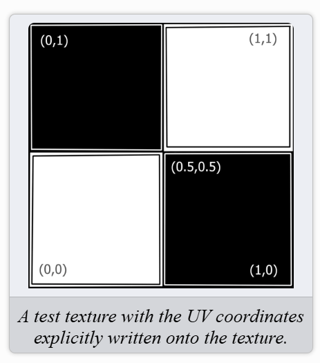
Likewise, every point in a geometry has a position in the 3D local space of the mesh. UV mapping, then, is the process of assigning 2D points in the texture to 3D points in the geometry.
For example, suppose the lips in the face model are at the point (0,0,0). We can see that the lips in the texture are close to the center, somewhere around (0.5,0.5).
So, we'll create a mapping:
Now, when we assign the texture as a color map in the material, the center of the texture will be mapped onto the lips.
Next, we must do the same for many other points in the geometry, assigning the ears, eyes, eyebrows, nose, and chin to the appropriate points of the texture. If this sounds like a daunting procedure, don't worry, because it's rare to do this manually.
For this model, the UV mapping was created in an external program, and in general, that's the recommended way to create UV mappings.
Data representing the UV mapping is stored on the geometry. The Three.js geometries like the BoxGeometry have already got UV mapping set up, and in most cases, when you load a model like a face that was created in an external program, it will also have UV mapping ready for use.
Once we have a geometry with a UV mapping, we can take any texture and apply it to the geometry and it will immediately work.
However, it might be hard to find other textures that will look good with a face model since the UV map must be carefully coordinated to match the texture to the correct points on the face, and doing this well is the work of a skilled 3D artist.
However, for simple shapes like a cube we can use nearly any image as a texture, turning the box into a wooden box, or a concrete box, or a crate, and so on.
Before we proceed with loading a texture and applying it to our cube, let's go over all the technical terms that we'll be using when working with textures.
We'll see the terms texture and image a lot in computer graphics literature. These are even often stored in the same format, such as PNG or JPG. What’s the difference?
The individual pixels that make up an image represent color. Another way of looking at this is that an image is a 2D array of colors.
In the early days of computer graphics, that was the case for textures too, but over time more and more uses were found for textures and now it's more correct to say that a texture is a 2D array of data.
This data can represent anything. Nowadays it's even possible to store geometry or animations in a texture.
When we use a texture in Three.js, we're usually using it to represent material properties like color, roughness, and opacity.
Textures are applied to a mesh by creating a Texture object and passing it to the map property of the material used to render the mesh.
Although technically incorrect, a texture is also often referred to as a map, or even a texture map, although map is most commonly used when assigning a texture to a material.
When using a texture to represent color, we'll say that we are assigning a texture to the color map slot on a material.
UV mapping is a method for taking a 2-dimensional texture and mapping it onto a 3-dimensional geometry.
Imagine a 2D coordinate system on top of the texture, with (0,0) in the bottom left and (1,1) in the top right. Since we already use the letters X, Y and Z for our 3D coordinates, we'll refer to the 2D texture coordinate using the letters U and V.
This is where the name UV mapping comes from.
Here's the formula used in UV mapping:
(u,v) represents a point on the texture, and (x,y,z) represents a point on the geometry, defined in local space. Technically, a point on a geometry is called a vertex.

In the figure above, the top left corner of the texture has been mapped to a vertex on the corner of the cube with coordinates (−1,1,1):
Similar mappings are done for the other five faces of the cube, resulting in one complete copy of the texture on each of the cube's six faces:
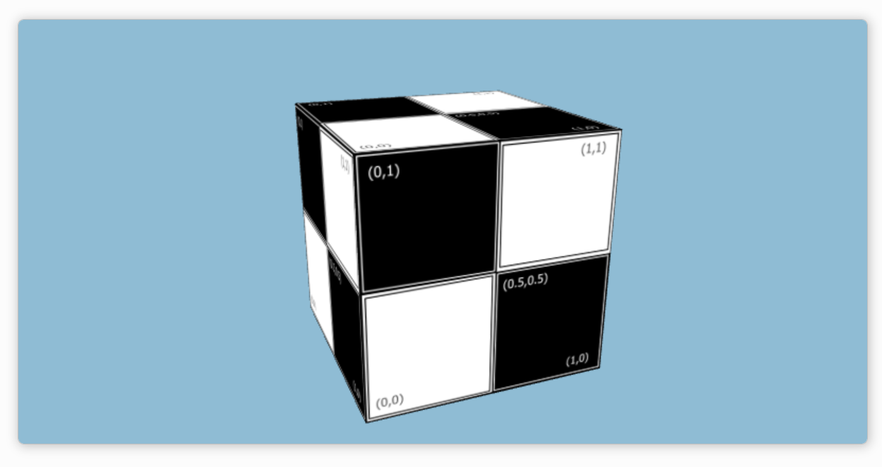
Note that there is no mapping for the point (0.5,0.5), the center of the texture. Only the corners of the texture are mapped, onto the eight corners of the cube, and the rest of the points are "guessed" from these.
By contrast, a complex model like a face must have many more UV coordinates defined to map the parts of the texture representing the nose, ears, eyes, lips, and so on, to the correct points of the geometry.
Fortunately, we rarely need to set up UV mapping manually since all the three.js geometries, including the BoxGeometry, have UV mapping built-in. We only need to load the texture and apply it to our material and everything will work.
Three.js has a built-in function TextureLoader() to load textures into your Three.js project.
First, we should create a loader:
const loader = new THREE.TextureLoader();Then we can load any texture or image by specifying its path in the load() function:
const texture = loader.load('path/to/texture.jpg');Now, we can apply the texture to the material by setting the map property of the material to the texture:
const material = new THREE.MeshStandardMaterial({ map: texture });Now, let's add a basic texture to our cube:
This is a basic image of a side of a wooden crate:
First, we should create a loader, then we can load our texture or image by specifying its path in the load() function.
const loader = new THREE.TextureLoader();
const texture = loader.load('https://raw.githubusercontent.com/amaraauguste/amaraauguste.github.io/refs/heads/master/courses/CISC3620/textures/crate.gif');
Now, we can apply the texture to the material by setting the map property of the material to the texture.
const material = new THREE.MeshStandardMaterial({ map: texture });And add a light source so we can actually see our crate:
//Create a AmbientLight
const light = new THREE.AmbientLight( 0xffffff, 1 );
scene.add(light);
Now, when we render the scene, we should see the cube with the crate texture applied to its surface.
Let's now create a crate positioned on a floor (plane)
First let's set our scene, camera, and renderer:
let width = 500;
let height = 400;
// Create the scene
const scene = new THREE.Scene();
scene.background = new THREE.Color("green"); //green screen to better view environment
const camera = new THREE.PerspectiveCamera(75, width / height, 0.1, 1000);
// Position the camera
camera.position.set(0, 3, 10); // Move it back on the z-axis and up on the y-axis

const renderer = new THREE.WebGLRenderer();
Now let's enable our renderer to include shadows:
renderer.shadowMap.enabled = true;And set size and add our renderer to view:
renderer.setSize(width, height);
document.body.appendChild(renderer.domElement); //add renderer to view
Don't forget our animate function:
function animate() {
    requestAnimationFrame(animate);
    renderer.render(scene, camera);
}
animate();
Now above our animate function, let's create a plane to act as our floor:
// Create plane geometry and material
const planeGeometry = new THREE.PlaneGeometry(50, 50);
const planeTexture = new THREE.TextureLoader().load('https://raw.githubusercontent.com/amaraauguste/amaraauguste.github.io/refs/heads/master/courses/CISC3620/textures/concrete%20floor.jpg');
const planeMaterial = new THREE.MeshStandardMaterial({ map: planeTexture });
const plane = new THREE.Mesh(planeGeometry, planeMaterial);
plane.rotation.x = -Math.PI / 2; // Rotate the plane to be horizontal
plane.receiveShadow = true; // Allow the plane to receive shadows
scene.add(plane);
Now let's create a crate to place on the floor:
// Create crate geometry and material
const geometry = new THREE.BoxGeometry(5, 5, 5);
const crateTexture = new THREE.TextureLoader().load('https://raw.githubusercontent.com/amaraauguste/amaraauguste.github.io/refs/heads/master/courses/CISC3620/textures/crate3.jpg');
const material = new THREE.MeshStandardMaterial({ map: crateTexture });

const crate = new THREE.Mesh(geometry, material);
crate.position.y = 2.5; // Position it above the plane
crate.castShadow = true; // Allow the cube to cast shadows
scene.add(crate);
Now when you run the code, you should see a cube positioned on a floor, however due to lack of lights it is hard to make out.
Now let's create a directional light so we can actually illuminate our scene:
const light = new THREE.DirectionalLight(0xffffff, 1);
light.position.set(7, 7, 7); // Position the light
light.castShadow = true; // Enable shadow casting for the light
scene.add(light);
Now we should see a cube textured to look like a wooden crate positioned on a concrete floor, illuminated by a directional light.
Let's add some orbit controls to take a closer look at the scene:
// Create orbit controls
const controls = new THREE.OrbitControls(camera, renderer.domElement);
controls.update();
It looks good but upon further inspection, notice how our floor texture looks more pixelated the closer we get. This is because the texture is being stretched over a large area.
One way to fix this is to increase the resolution of the texture. However, this can be expensive in terms of memory and performance.
Another way to fix this is to use a technique called texture tiling. Texture tiling involves repeating the texture multiple times over the surface of the mesh.
Let's add texture tiling to our floor:
//to improve by repeating texture
planeTexture.wrapS = THREE.RepeatWrapping; // Repeat the texture in the x-direction
planeTexture.wrapT = THREE.RepeatWrapping; // Repeat the texture in the y-direction
planeTexture.repeat.set(4, 4); // Repeat the texture 4 times in both directions
Now we see the floor texture repeated multiple times over the surface of the plane, which improves the appearance of the texture.
So far, we've learned how to create a scene, add objects to it, add lights, cast shadows, and apply textures to those objects.
For example, we've played around with cubes but if we want realistic scenes that are not just made up of crates and boxes we need to start building more complex objects.
Let's say we want to create a table. What does a table actually look like?
A basic table has a flat surface and four legs. How can we create this in Three.js?
One way to do this is to use primitive geometries like BoxGeometry to create custom models.
For example, to create a table, we can use a BoxGeometry for the table top and four additional BoxGeometries for the legs.
First, let's set up our scene:
let width = 500;
let height = 400;
// Create the scene
const scene = new THREE.Scene();
const camera = new THREE.PerspectiveCamera(75, width / height, 0.1, 1000);
// Position the camera
camera.position.z = 10; // Move it back on the z-axis
camera.position.y = 2; // Move it up on the y-axis
const renderer = new THREE.WebGLRenderer();
renderer.shadowMap.enabled = true; // Enable shadows in the renderer
renderer.setSize(width, height);
renderer.antialias = true; // Enable antialiasing
document.body.appendChild(renderer.domElement); //add renderer to view
Let's also add orbit controls so we can get a better view of our scene:
// Create orbit controls
const controls = new THREE.OrbitControls(camera, renderer.domElement);
controls.update();
And don't forget our animate() function so we can actually see our scene:
function animate() {
    requestAnimationFrame(animate);
    renderer.render(scene, camera);
}
animate();
Let's add a floor for our objects to sit atop:
// Create a floor that receives shadows
const floorGeometry = new THREE.PlaneGeometry(20, 20);
const floorMaterial = new THREE.MeshBasicMaterial({ color: "gray" });
const floor = new THREE.Mesh(floorGeometry, floorMaterial);
floor.rotation.x = -Math.PI / 2; // Rotate the floor to be horizontal
floor.position.y = -2;
floor.receiveShadow = true;
scene.add(floor);
Now let's actually create our table. First we need a table top:
// Create table top geometry and material
const tableTopGeometry = new THREE.BoxGeometry(8.5, 0.75, 4); //width, height, depth
const tableTopMaterial = new THREE.MeshBasicMaterial({ color: "brown" });
const tableTop = new THREE.Mesh(tableTopGeometry, tableTopMaterial);
tableTop.position.y = 0.85; // Position the table top above the floor
tableTop.castShadow = true; // Allow the table top to cast shadows
scene.add(tableTop);
Now let's create the legs of the table:
const legGeometry = new THREE.BoxGeometry(0.5, 3, 0.5); //width, height, depth
const legMaterial = new THREE.MeshBasicMaterial({ color: "brown" });
const leg1 = new THREE.Mesh(legGeometry, legMaterial);
const leg2 = new THREE.Mesh(legGeometry, legMaterial);
const leg3 = new THREE.Mesh(legGeometry, legMaterial);
const leg4 = new THREE.Mesh(legGeometry, legMaterial);
leg1.position.set(-4, -1, 1.75); // Position the legs at the corners of the table top
leg2.position.set(-4, -1, -1.75);
leg3.position.set(4, -1, 1.75);
leg4.position.set(4, -1, -1.75);
leg1.castShadow = true;
leg2.castShadow = true;
leg3.castShadow = true;
leg4.castShadow = true;
scene.add(leg1, leg2, leg3, leg4);
This is okay but what if we needed to reposition the table now? Because we added each part of the table to the scene as it's own individual object, we would have to manually adjust the position of each leg. This is not ideal.
Instead of adding each part of the table as a separate object, we can group them together using a Group object.
Let's group the table top and legs together:
// Create a group to hold the table top and legs
const table = new THREE.Group();
table.add(tableTop, leg1, leg2, leg3, leg4);
scene.add(table);
Now, when we want to move the table, we can simply move the table object and all of its children will move with it.
Let's better position the table so the legs are not going through the floor:
table.position.y = 0.5;We should now have a simple table in our scene. We can add more objects to the scene in a similar way to create more complex scenes.
Notice that we used MeshBasicMaterial since we did not set up any lights. Let's fix that:
First, we need to change our material to something that uses lights, i.e MeshStandardMaterial.
When we change the material of the table, we should see a simple black silhouette of the brown table we once had. Don't worry we will see it again once we add light.
Now, let's add some light:
// Create a directional light
const light = new THREE.DirectionalLight("white", 1);
light.position.set(7, 7, 7);
light.castShadow = true;

// Add the light to the scene
scene.add(light);
Now we should see a table with legs positioned on a floor, illuminated by a directional light.
Let's make sure to update our floor material as well. Now we should see a shadow of the table being cast onto the floor.
Our table looks good but it's a bit plain. Let's add a texture to the table top:
First, let's load our texture:
// Create a texture loader
const loader = new THREE.TextureLoader();
const tableTexture = loader.load('https://raw.githubusercontent.com/amaraauguste/amaraauguste.github.io/refs/heads/master/courses/CISC3620/textures/wood%20table%20top%20texture.jpg');
Now, let's apply the texture to the table top:
const tableTopMaterial = new THREE.MeshStandardMaterial({ map: tableTexture });And do the same to the legs:
const legMaterial = new THREE.MeshStandardMaterial({ map: tableTexture });Now our table should have a wooden texture applied to the table top and legs and look more realistic.
In addition to our standard primitive geometries like BoxGeometry and PlaneGeometry, Three.js also provides a number of built-in geometries for creating more complex objects, for example: TeapotGeometry
We'll add a teapot to our scene but first let's understand TeapotGeometry:
TeapotGeometry is a geometry that represents a teapot. It's a complex geometry that is not built into Three.js by default, but we can add it by importing it from the Three.js examples.
TeapotGeometry has multiple parameters that can be set to customize the teapot, such as size, segments, and detail.
However, the only required parameter is the size of the teapot.
We need to add the following script to our HTML file to import the TeapotGeometry:
<script src="https://cdn.jsdelivr.net/npm/three@0.128.0/examples/js/geometries/TeapotGeometry.js"></script>Now we can create a teapot and add it to our scene:
// Create teapot geometry and material
const teapotGeometry = new THREE.TeapotGeometry(0.75); // Set the size of the teapot
const teapotMaterial = new THREE.MeshStandardMaterial({ color: "white" });
const teapot = new THREE.Mesh(teapotGeometry, teapotMaterial);
teapot.position.y = 2.5; // Position the teapot to sit atop the table
teapot.castShadow = true;
scene.add(teapot);
We should now see a white teapot sitting atop our wooden table. However, there is no shadow on the table from our teapot. This is because although we have enable shadow casting for the teapot, we have not enabled shadow receiving for the table top.
Let's enable shadow receiving for the table top:
// Enable shadow receiving for the table
tableTop.receiveShadow = true;
Now we should see a shadow of the teapot being cast onto the table.
Now we have a simple scene with a table and a teapot. We can add more objects to the scene in a similar way to create more complex scenes.
Let's add texture to our floor:
const floorTexture = loader.load('https://raw.githubusercontent.com/amaraauguste/amaraauguste.github.io/refs/heads/master/courses/CISC3620/textures/wood%20floor.jpg');And remember to update our floorMaterial to apply the texture:
const floorMaterial = new THREE.MeshStandardMaterial({ map: floorTexture });And now our scene looks more realistic than it did when we began!
We can modify this scene by adding more objects, such as walls, furniture, lights, etc.
Let's create walls for our scene so we have a room. We will only need three walls as the fourth will be occupied by our camera.
First, let's create a wall:
// Create wall geometry and material
const wallGeometry = new THREE.PlaneGeometry(20, 15);
const wallMaterial = new THREE.MeshStandardMaterial({ color: "#a0d6b4" }); // Turquoise Green
const wall = new THREE.Mesh(wallGeometry, wallMaterial);
wall.position.z = -10; // Position the wall behind the table
wall.position.y = 5.5; // Position the wall at the same height as the table
wall.receiveShadow = true; // Allow the wall to receive shadows
scene.add(wall);
We need to ensure that the wall has two sides or else we will only see the wall from one side. We can do this by setting the side property of the material to THREE.DoubleSide:
wall.material.side = THREE.DoubleSide;While on the topic, let's also make sure our floor has two sides:
floor.material.side = THREE.DoubleSide;Now we should see a turquoise green wall behind our table. Let's add two more walls:
const wall2 = wall.clone(); // Clone the wall
wall2.rotation.y = Math.PI / 2; // Rotate the wall to be perpendicular to the first wall
wall2.position.x = -10; // Position the wall to the left of the table
wall2.position.z = 0.0001; // Position so edges of the walls meet
scene.add(wall2);

const wall3 = wall.clone();
wall3.rotation.y = Math.PI / 2; // Rotate the wall to be perpendicular to the first wall
wall3.position.x = 10; // Position the wall to the right of the table
wall3.position.z = 0.0001; // Position so edges of the walls meet
scene.add(wall3);
Now how our right wall is shadowed, that is due to lack of light on that side. Let's add a point light above (like a ceiling light) to view better:
// Create a point light
const light2 = new THREE.PointLight("white", 1);
light2.position.set(0, 20, 0);
light2.castShadow = true;
scene.add(light2);
Now our scene should be more illuminated.
How does having these two different lights in different positions affect our scene? How does it affect our shadows?
What does our scene look like if we rid of our directional light? How does having just the center point light change the scene?
If our teapot's shadow looks a bit blocky from the point light, we can fix this by applying some antialiasing:
// Antialias the point light shadow
light2.shadow.mapSize.width = 2048; // Increase shadow map size for better quality
light2.shadow.mapSize.height = 2048;
light2.shadow.radius = 4; // Increase shadow radius for softer shadows
This should make our shadow look smoother.
And there we have it! We've used what we've learned so far to build a more complex scene with a table, teapot, walls, and lights.
Now think about tables that we have seen in reality, they can vary from material. A standard table like our object can be made out of wood (like our example), marble (for which we would use a different texture and a shinier material), or even glass.
Let's talk about the properties of glass.
Glass is transparent, meaning light can pass through it. This is different from our current table material which is opaque, meaning light cannot pass through it.
In order to create transparent objects, first we need to set the transparent property of our material to true. We also need to set the opacity property to a value between 0 and 1, where 0 is completely transparent and 1 is completely opaque.
Let's create a glass table:
const tableMaterial = new THREE.MeshPhongMaterial({ color : "pink",
    transparent : true,
    opacity: 0.75
}); //opacity will not work if transparent is not set to true
Now we should see a pink glass table in our scene.
Let's add a GUI to toggle our lights on and off:
First, we need to add the following script to our HTML file to import the GUI library:
<script src="https://cdn.jsdelivr.net/npm/dat.gui/build/dat.gui.min.js"></script>Now we can create a GUI to toggle our lights on and off:
// GUI setup
const gui = new dat.GUI();
const guiParams = {
    directionalLight: true, // Directional light toggle
    pointLight: true, // Point light toggle
};
Now we can add controls to our GUI to toggle our lights:
gui.add(guiParams, 'directionalLight').name('Directional Light').onChange((value) => {
    light.visible = value;
});

gui.add(guiParams, 'pointLight').name('Point Light').onChange((value) => {
    light2.visible = value;
});
Now we should see a GUI with toggles for our directional and point lights.
Let's try a different scene, a tree on some grass.
Let's set our scene:
// Scene setup
let width = 500;
let height = 400;
const scene = new THREE.Scene();
scene.background = new THREE.Color("skyblue"); // Set sky color

const camera = new THREE.PerspectiveCamera(75, width / height, 0.1, 1000);
const renderer = new THREE.WebGLRenderer();
renderer.setSize(width, height);
renderer.shadowMap.enabled = true;
renderer.antialias = true;
document.body.appendChild(renderer.domElement);

// Camera position
camera.position.set(0, 1, 10); // Set camera position so we can view the scene

// Add OrbitControls to enable mouse movement
const controls = new THREE.OrbitControls(camera, renderer.domElement);
controls.update();


function animate() {
    requestAnimationFrame(animate);
    renderer.render(scene, camera);
}
animate();
And ensure that we have an light source:
// Create a directional light
const light = new THREE.DirectionalLight("white", 1);
light.position.set(-10, 7, 7);
light.castShadow = true;
scene.add(light);
Now we need our grass ground:
// Create grass geometry and material
const groundGeometry = new THREE.PlaneGeometry(100, 100);
const groundMaterial = new THREE.MeshStandardMaterial({ color: "green", side: THREE.DoubleSide });
const ground = new THREE.Mesh(groundGeometry, groundMaterial);
ground.rotation.x = -Math.PI / 2; // Rotate to make it flat
ground.receiveShadow = true;
scene.add(ground);
And now we'll write a function to make a pine tree. First, think about how a pine tree looks. A standard one has a triangular shape with a brown trunk and green leaves. We can create this using a ConeGeometry for the leaves and a CylinderGeometry for the trunk.
Let's create a pine tree:
// Function to create a pine tree
function createPineTree() {
    const tree = new THREE.Group(); // Group to hold tree components

    // Create the trunk of the tree
    const trunkGeometry = new THREE.CylinderGeometry(0.1, 0.25, 2, 8); // Radius top, radius bottom, height, number of segments
    const trunkMaterial = new THREE.MeshStandardMaterial({ color: "brown" }); // Brown color for the trunk
    const trunk = new THREE.Mesh(trunkGeometry, trunkMaterial);
    trunk.castShadow = true;
    trunk.position.y = 0.5;  // Position trunk at the bottom of the tree
    tree.add(trunk);  // Add trunk to the tree group

    // Create foliage using cones
    const foliageGeometry = new THREE.ConeGeometry(0.8, 1.5, 8); // Radius, height, number of segments
    const foliageMaterial = new THREE.MeshStandardMaterial({ color: "green" }); // Green color for foliage

    // Create multiple layers of foliage for a better shape
    for (let i = 0; i < 3; i++) {
        const foliage = new THREE.Mesh(foliageGeometry, foliageMaterial);
        foliage.position.y = 1 + i * 0.5;  // Adjust position for layers
        foliage.rotation.y = Math.random() * Math.PI;  // Random rotation
        foliage.castShadow = true;
        tree.add(foliage);  // Add foliage layer to tree
    }

    return tree;  // Return the complete tree object
}
Now we can add our pine tree to the scene:
// Create a pine tree
const pineTree = createPineTree();
pineTree.scale.set(2,2,2); // Scale the tree to make it larger
pineTree.position.y = 1; // Position the tree above the ground
pineTree.position.x = -5; // Position the tree to the left
scene.add(pineTree);
Now we should see a pine tree (and it's shadow) on some grass in our scene.
Let's add a simple house next to the tree:
// Create a simple house
const houseStructure = new THREE.Group(); // to group all our objects
const houseGeometry = new THREE.BoxGeometry(4, 4, 4);
const houseMaterial = new THREE.MeshStandardMaterial({ color: 0xffcc00 });
const house = new THREE.Mesh(houseGeometry, houseMaterial);
house.castShadow = true;
house.position.set(0, 2, 0);
houseStructure.add(house);

// Create a simple roof for the house
const roofGeometry = new THREE.ConeGeometry(2.8, 2, 4);
const roofMaterial = new THREE.MeshStandardMaterial({ color: 0x8B0000 });
const roof = new THREE.Mesh(roofGeometry, roofMaterial);
roof.castShadow = true;
roof.position.set(0, 5, 0);
roof.rotation.y = Math.PI / 4; // Rotate to place it correctly on top of the house
houseStructure.add(roof);

// Create a door for the house
const doorGeometry = new THREE.BoxGeometry(1, 2, 0.1);
const doorMaterial = new THREE.MeshStandardMaterial({ color: 0x654321 }); // Door color
const door = new THREE.Mesh(doorGeometry, doorMaterial);
door.position.set(0, 1, 2); // Position the door
houseStructure.add(door);

// Create windows for the house
const windowGeometry = new THREE.BoxGeometry(1, 1, 0.1);
const windowMaterial = new THREE.MeshPhongMaterial({ color: 0xadd8e6 }); // Window color

// Left window
const leftWindow = new THREE.Mesh(windowGeometry, windowMaterial);
leftWindow.position.set(-1.25, 2, 2); // Position left window
houseStructure.add(leftWindow);

// Right window
const rightWindow = new THREE.Mesh(windowGeometry, windowMaterial);
rightWindow.position.set(1.25, 2, 2); // Position right window
houseStructure.add(rightWindow);

scene.add(houseStructure);
Let's move the house forward a bit:
houseStructure.position.z = 2;And we should move out camera back on the z-axis to reflect this.
Now we should see a pine tree, a house, and some grass in our scene.
Let's add a GUI to toggle our objects on and off:
const gui = new dat.GUI();
const guiParams = {
    tree: true, // Tree toggle
    house: true, // House toggle
};

gui.add(guiParams, 'tree').name('Pine Tree').onChange((value) => {
    pineTree.visible = value;
});

gui.add(guiParams, 'house').name('House').onChange((value) => {
    houseStructure.visible = value;
});
Now we should be able to toggle our pine tree and house visible by our GUI.
Let's modify our house with some textures for the base, roof, and door.
Let's create our texture loader:
// Create a texture loader
const loader = new THREE.TextureLoader();
Now let's load our textures:
const houseTexture = loader.load('https://raw.githubusercontent.com/amaraauguste/amaraauguste.github.io/refs/heads/master/courses/CISC3620/textures/brown%20house%20texture.jpg');
const roofTexture = loader.load('https://raw.githubusercontent.com/amaraauguste/amaraauguste.github.io/refs/heads/master/courses/CISC3620/textures/red%20roof%20texture.png');
const doorTexture = loader.load('https://raw.githubusercontent.com/amaraauguste/amaraauguste.github.io/refs/heads/master/courses/CISC3620/textures/pixel_door.png');
Now let's apply the textures to our house:
const houseMaterial = new THREE.MeshStandardMaterial({ map: houseTexture });
const roofMaterial = new THREE.MeshStandardMaterial({ map: roofTexture });
const doorMaterial = new THREE.MeshStandardMaterial({ map: doorTexture });
And now our house should have textures applied to the base, roof, and door.
Let's improve our roof with some texture tiling:
roofTexture.wrapS = THREE.RepeatWrapping; // Repeat the texture in the x-direction
roofTexture.wrapT = THREE.RepeatWrapping; // Repeat the texture in the y-direction
roofTexture.repeat.set(4, 4); // Repeat the texture 4 times in both directions
Now our roof should have a tiled texture applied to it.
And there we have it! We've used what we've learned so far to successfully build a more complex (although still rather simple) scene both indoors and outdoors.
So far, we've used primitive geometries like BoxGeometry, ConeGeometry, and CylinderGeometry to create objects in Three.js.
However, sometimes we may want to create custom geometries that are not built into Three.js.
We've seen a bit of this with BufferGeometry, which allows us to create custom geometries by specifying the vertices and faces of the geometry.
Another way to create custom geometries is to use the THREE.Shape class
First, we need to define the shape. We can do this by creating a path using the THREE.Shape class.
The THREE.Shape class allows us to define 2D shapes by specifying a series of points. This is similar to how we define paths in SVG, Adobe Illustrator, or like we did in HTML5 Canvas.
Let's create a custom geometry using THREE.Shape:
const tri = new THREE.Shape();
tri.moveTo(0, 1);
tri.lineTo(1, -1);
tri.lineTo(-1, -1);
We've created a triangle shape with vertices at (0, 1), (1, -1), and (-1, -1).
Now we can create a custom geometry using the shape:
const geometry = new THREE.ShapeGeometry(tri);THREE.ShapeGeometry() takes a shape as a parameter and creates a geometry based on that shape. We can then create a mesh using the custom geometry and a material and add it to the scene.
const material = new THREE.MeshStandardMaterial({ color: "blue" });
const mesh = new THREE.Mesh(geometry, material);
scene.add(mesh);
Now we should see a blue triangle in our scene.
We can create a variety of custom geometries by defining different shapes and paths.
Another way to create custom geometries is to use ExtrudeGeometry.
ExtrudeGeometry allows us to create geometries by extruding a 2D shape along a path in 3D space. This is similar to how we create 3D objects by extruding 2D shapes in 3D modeling software.
ExtrudeGeometry is useful for creating complex geometries like buildings, furniture, and other objects with depth.
Let's extrude our triangle to create a pyramid:
const extrudeSettings = {
    steps: 1, // Number of steps to extrude the shape
    depth: 1, // Depth of the extrusion
    bevelEnabled: false, // Disable beveling
};

const pyramidGeometry = new THREE.ExtrudeGeometry(tri, extrudeSettings);
const pyramidMaterial = new THREE.MeshStandardMaterial({ color: "red" });
const pyramidMesh = new THREE.Mesh(pyramidGeometry, pyramidMaterial);
scene.add(pyramidMesh);
ExtrudeGeometry takes two parameters: the shape we want to extrude and extrusion settings.
Extrusion settings include:
Let's create a custom cube:
const shape = new THREE.Shape();
shape.moveTo(0, 0); // Move to the starting point
shape.lineTo(0, 1); // Draw a line to the next point
shape.lineTo(1, 1); // Draw a line to the next point
shape.lineTo(1, 0); // Draw a line to the next point
shape.lineTo(0, 0); // Draw a line back to the starting point
Now we can create our custom geometry using ExtrudeGeometry:
const extrudeSettings = {
    steps: 2,
    depth: 1,
    bevelEnabled: false, // Disable beveling which creates rounded edges
};

const geometry = new THREE.ExtrudeGeometry(shape, extrudeSettings);
Now we can create a mesh using our custom geometry:
const material = new THREE.MeshStandardMaterial({ color: "red" });
const mesh = new THREE.Mesh(geometry, material);
scene.add(mesh);
Now we should see a red extruded shape (cube) in our scene.
For example, we can create a custom geometry by extruding a star shape:
// Create a star shape
const starShape = new THREE.Shape();
starShape.moveTo(0, 0.5);
starShape.lineTo(0.15, 0.15);
starShape.lineTo(0.5, 0.15);
starShape.lineTo(0.2, -0.15);
starShape.lineTo(0.3, -0.5);
starShape.lineTo(0, -0.25);
starShape.lineTo(-0.3, -0.5);
starShape.lineTo(-0.2, -0.15);
starShape.lineTo(-0.5, 0.15);
starShape.lineTo(-0.15, 0.15);
starShape.lineTo(0, 0.5);

// Extrude the star shape
const extrudeSettings = {
    steps: 2,
    depth: 0.1,
    bevelEnabled: false,
};

const starGeometry = new THREE.ExtrudeGeometry(starShape, extrudeSettings);
const starMaterial = new THREE.MeshStandardMaterial({ color: "yellow" });
const starMesh = new THREE.Mesh(starGeometry, starMaterial);
starMesh.scale.set(4,4,4);
scene.add(starMesh);
Now we should see a yellow extruded star shape in our scene.
Or let's create a simple heart shape.
To draw a heart shape, we need to define a series of points that form the shape of a heart. The easiest way to do this is with bezier curves.
To refresh your memory, a bezier curve is a parametric curve that is defined by a set of control points. In Three.js (like in HTML5 Canvas), we can use the bezierCurveTo() method of the Shape class to create bezier curves.
The parameters of bezierCurveTo() are the x and y coordinates of the control point and the x and y coordinates of the end point of the curve.
const heartShape = new THREE.Shape();
heartShape.moveTo( 2.5, 2.5 );
heartShape.bezierCurveTo( 2.5, 2.5, 2.0, 0, 0, 0 );
heartShape.bezierCurveTo( - 3.0, 0, - 3.0, 3.5, - 3.0, 3.5 );
heartShape.bezierCurveTo( - 3.0, 5.5, - 1.0, 7.7, 2.5, 9.5 );
heartShape.bezierCurveTo( 6.0, 7.7, 8.0, 5.5, 8.0, 3.5 );
heartShape.bezierCurveTo( 8.0, 3.5, 8.0, 0, 5.0, 0 );
heartShape.bezierCurveTo( 3.5, 0, 2.5, 2.5, 2.5, 2.5 );

const extrudeSettings = {
    steps: 2,
    depth: 1,
    bevelEnabled: true,
};
const geometry = new THREE.ExtrudeGeometry( heartShape, extrudeSettings );
geometry.rotateX(Math.PI * 1);
geometry.center();

const material = new THREE.MeshStandardMaterial({color: "#FF69B4"});

const heartMesh = new THREE.Mesh( geometry, material);

heartMesh.scale.set(0.25, 0.25, 0.25);

scene.add(heartMesh);
It's starting to come along but it's not quite right. We can adjust even further to get the shape we're after:
const extrudeSettings = {
    steps: 2,
    depth: 1,
    bevelEnabled: true,
    curveSegments: 40, // Number of points on the curves
    bevelSegments: 20, // Number of segments for the bevel
    bevelThickness: 0.75, // Thickness of the bevel
    bevelSize: 0.75 // Size of the bevel
};
These modifications should give us a more accurate heart shape by adding more curve segments and bevel segments to the extrusion.
Now we should see a pink extruded heart shape in our scene.
We can also "punch" a shaped hole into other shapes.
const tri = new THREE.Shape();
tri.moveTo(0, 2);
tri.lineTo(2, -2);
tri.lineTo(-2, -2);
// add the hole
const hole = new THREE.Shape();
hole.arc(0, -0.8, 1.0, 0, Math.PI * 2);

tri.holes.push(hole); // push to the shapes holes array

const extrudeSettings = {
    steps: 2,
    depth: 1,
    bevelEnabled: false
};
const geometry = new THREE.ExtrudeGeometry(tri, extrudeSettings);
geometry.rotateX(Math.PI * 1);
geometry.center();

const mesh = new THREE.Mesh(geometry, new THREE.MeshNormalMaterial());

scene.add(mesh);
This code creates a triangle with a hole in the center. The hole is created by adding a circle shape to the triangle's holes array and extruding the shape with the hole.
We can also create custom geometries by setting the vertices of the geometry directly using the setFromPoints method of the Shape class.
We can set the state of a path by way of an array of THREE.vector2 class objects. The Vector2 class is a class that is used to represent a point in 2D space.
We can create an array of these Vector2 objects by any means that we would like, and then we can just create a shape, and then call the set from points method off of the shape and pass the array of Vector2 objects.
// creating an array of THREE.Vector2 objects
const points = []; // array to hold the points
const len = 100;
let i = 0;
while(i < len){ // loop to create the points
    const a = i / len;
    const x = -3  + 6 * a; // x position that will be used to create a parabola
    const y = Math.sin( Math.PI * 1.0 * a ) * 4; //to create a parabola
    points.push(new THREE.Vector2(x, y));
    i += 1;
}
const shape = new THREE.Shape();
// creating the path by using the set from points method with the array of THREE.Vector2 objects
shape.setFromPoints(points);

const extrudeSettings = {
    steps: 2,
    depth: 1.5,
    bevelEnabled: false
};
const geometry = new THREE.ExtrudeGeometry( shape, extrudeSettings );
geometry.center(); //to center the geometry

const material = new THREE.MeshStandardMaterial({ color: "blue" });
const mesh = new THREE.Mesh( geometry, material );

scene.add(mesh);
And there we have it! We've used what we've learned so far to create custom geometries using THREE.Shape and ExtrudeGeometry.
Now think about what other custom geometries you could create using these methods. What shapes could you create? What objects could you model?
What other methods could you use to create custom geometries in Three.js?
What are some other ways you could modify the custom geometries we've created?
What are some other ways you could use custom geometries in your Three.js projects?
So far we've created geometries using Three.js's built-in geometries and custom geometries.
But as aforementioned the 3D Graphics pipeline actually starts with a 3D model. A 3D model is a digital representation of a 3D object or scene.
To create beautiful 3D models, a sophisticated modeling program is required, like Blender, Maya, 3ds Max, or SketchUp. We can use Three.js to build any kind of 3D application, however, building a modeling app from scratch would be a huge amount of work. A much simpler solution is to use an existing program and export your work for use in Three.js ... or, "cheat", and download any of the millions of amazing models and other scene assets that are available for free in many places around the web.
Once a 3D model is created, it can be exported to a file format that can be read by a 3D graphics library like Three.js.
Three.js supports a variety of 3D model file formats including:
Let's talk about each of these formats:
OBJ (Wavefront) is a simple text-based file format that stores information about the 3D model's geometry, materials, and textures.
glTF (GL Transmission Format) is a binary file format that stores information about the 3D model's geometry, materials, textures, and animations. GLTF is designed to be compact and efficient for web-based 3D applications.
FBX (Filmbox) is a proprietary file format developed by Autodesk that stores information about the 3D model's geometry, materials, textures, animations, and other data. FBX is widely used in the film and game industry.
DAE (Collada) is an XML-based file format that stores information about the 3D model's geometry, materials, textures, animations, and other data. Collada is designed to be an open and interoperable format for 3D content.
STL (Stereolithography) is a file format that stores information about the 3D model's geometry as a series of triangles. STL is commonly used for 3D printing and rapid prototyping.
3DS (3D Studio) is a file format developed by Autodesk that stores information about the 3D model's geometry, materials, textures, and animations. 3DS is widely used in the film and game industry.
PLY (Polygon File Format) is a file format that stores information about the 3D model's geometry as a series of vertices, edges, and faces. PLY is commonly used for 3D scanning and computer graphics research.
There have been many attempts at creating a standard 3D asset exchange format over the last thirty years or so. FBX, OBJ (Wavefront) and DAE (Collada) formats were the most popular of these until recently, although they all have problems that prevented their widespread adoption.
For example, OBJ doesn't support animation, FBX is a closed format that belongs to Autodesk, and the Collada spec is overly complex, resulting in large files that are difficult to load.
However, recently, a newcomer called glTF has become the de facto standard format for exchanging 3D assets on the web. glTF (GL Transmission Format), sometimes referred to as the JPEG of 3D, was created by the Kronos Group, the same people who are in charge of WebGL, OpenGL, and a whole host of other graphics APIs.
Originally released in 2017, glTF is now the best format for exchanging 3D assets on the web, and in many other fields. In this class, we will always use glTF, and if possible, you should do the same. It's designed for sharing models on the web, so the file size is as small as possible and your models will load quickly.
glTF files can contain models, animations, geometries, materials, lights, cameras, or even entire scenes. This means you can create an entire scene in an external program then load it into Three.js.
glTF files come in standard and binary form. These have different extensions:
Both standard and binary glTF files may contain textures embedded in the file or may reference external textures. Since binary .glb files are considerably smaller, it's best to use this type. On the other hand, uncompressed .gltf are easily readable in a text editor, so they may be useful for debugging purposes.
Now that we know about the different types of 3D model file formats, let's learn how to load a 3D model into a Three.js scene.
We'll start with three simple and beautiful models of a parrot, a flamingo, and a stork, created by the talented people at mirada.com. These three models are low poly, meaning they'll run on even the most low-power of mobile devices, and they are even animated.
We will load Parrot.glb, Flamingo.glb, and Stork.glb and then add the bird-shaped meshes each file contains to our scene. Later, we will learn how to play the flying animation that is included with each bird.
In order to load a 3D model into Three.js, we need to use a loader. A loader is a class that reads a 3D model file and creates a Three.js object from it. More specifically, since we're using glTF models, we'll use the GLTFLoader class.
Since glTF is relatively new, your favorite application might not have an exporter yet. In that case, you can convert your models to glTF before using them, or use another loader such as the FBXLoader or OBJLoader. All Three.js loaders work the same way, so if you do need to use another loader, everything will still apply, with only minor differences.
To load glTF files, first, we need to add the GLTFLoader plugin to our environment. This works the same way as adding the OrbitControls plugin:
<script src="https://cdn.jsdelivr.net/npm/three@0.128.0/examples/js/loaders/GLTFLoader.js"></script>Now we can now create an instance of the GLTFLoader class:
const loader = new THREE.GLTFLoader();Next, we can use the load() method of the loader to load a glTF model file:
loader.load('https://raw.githubusercontent.com/amaraauguste/amaraauguste.github.io/master/courses/CISC3620/models/Parrot.glb', function (gltf) {
    const parrot = gltf.scene;
    scene.add(parrot);
});
The load() method takes two parameters: the URL of the model file and a callback function that is called when the model is loaded. The callback function receives a gltf object that contains the loaded 3D model. We can access the 3D model scene by using gltf.scene and then add it to our Three.js scene.
Let's add the stork and flamingo models to our scene:
loader.load('https://raw.githubusercontent.com/amaraauguste/amaraauguste.github.io/master/courses/CISC3620/models/Stork.glb', function (gltf) {
    const stork = gltf.scene;
    scene.add(stork);
});

loader.load('https://raw.githubusercontent.com/amaraauguste/amaraauguste.github.io/master/courses/CISC3620/models/Flamingo.glb', function (gltf) {
    const flamingo = gltf.scene;
    scene.add(flamingo);
});
It is possible for models loaded from a glTF file to have a position already specified, but that's not the case here, so all three models start at the point (0,0,0), all jumbled together on top of each other.
We'll adjust the position of each bird to make it look like they are flying in formation:
parrot.position.set(0, 20, 2.5); //before we add the parrot to the scene
stork.position.set(70, -40, -10); //before we add the stork to the scene
flamingo.position.set(-70, 0, -10); //before we add the flamingo to the scene
Now the birds should be in a more visually appealing formation.
We will revisit these birds later but first let's pivot back to stationary objects like furniture.
If you are interested in creating your own 3D models, you can start by learning how to use one of these software programs. However, for those who are not interested in creating their own 3D models, there are many websites that offer free and paid 3D models that you can download and use in your projects.
Some of these include:
We'll use 3D models from Poly Pizza in this class, as they offer a variety of free 3D models that we can use in our projects as long as we credit the creator under the Creative Commons license. However you can use any of the above websites to find 3D models for your projects or create your own.
Let's load a glTF model of a table from Poly Pizza into our scene:
 // Load GLB Table Model
const loader = new THREE.GLTFLoader();
//Model Credit: Table Round Small by Quaternius
loader.load('https://raw.githubusercontent.com/amaraauguste/amaraauguste.github.io/master/courses/CISC3620/models/Table%20Round%20Small.glb', function (gltf) {
    const tableModel = gltf.scene;
    tableModel.scale.set(20, 20, 20); // Scale the model
    tableModel.position.y = -9.5; // Position the model
    scene.add(tableModel);
});
Now we should see a 3D model of a table in our scene.
Apart from transformations like scaling up (or down) the model we can also adjust how the model looks by changing the material of the model.
Let's change the material of the table model as we like it:
// Load GLB Table Model
const loader = new THREE.GLTFLoader();
//Model Credit: Table Round Small by Quaternius
loader.load('https://raw.githubusercontent.com/amaraauguste/amaraauguste.github.io/master/courses/CISC3620/models/Table%20Round%20Small.glb', function (gltf) {
    const tableModel = gltf.scene;
    tableModel.scale.set(20, 20, 20); // Adjust table model scale if needed
    tableModel.position.y = -9.5; // Adjust table model position if needed
    const tableMaterial = new THREE.MeshStandardMaterial({ color: "white" });
    tableModel.traverse((child) => {
        if (child.isMesh) {
            child.material = tableMaterial;
            child.castShadow = true; // The table will cast shadows
            child.receiveShadow = true; // The table will receive shadows
        }
    });

    scene.add(tableModel);
});
This code creates a new MeshStandardMaterial with a white color and then uses the traverse() method to iterate over all the child objects of the table model. For each child object that is a mesh, it sets the material to the new material.
Now we should see a white table model in our scene.
Let's add another model, a flower pot, to sit on the table:
// Load GLB Flower Pot Model
const loader2 = new THREE.GLTFLoader();
//Model Credit: Flower by jeremy [CC-BY] via Poly Pizza
loader2.load('https://raw.githubusercontent.com/amaraauguste/amaraauguste.github.io/master/courses/CISC3620/models/Flower.glb', function (gltf) {
    const flowerPotModel = gltf.scene;
    flowerPotModel.scale.set(20, 20, 20); // Adjust flower pot model scale if needed
    flowerPotModel.position.y = -5; // Adjust flower pot model position if needed
    // Set shadow properties
    flowerPotModel.traverse((child) => {
        if (child.isMesh) {
            child.castShadow = true; // The flower pot will cast shadows
            child.receiveShadow = true; // The flower pot can receive shadows
        }
    });

    scene.add(flowerPotModel);
});
This code loads a GLTF model of a flower pot and adds it to the scene. We can adjust the scale and position of the flower pot model as needed.
Now we should see a flower pot model on the table in our scene.
Let's group the models together so they are easier to reposition:
// Create a group to hold the table and flower pot models
const modelsGroup = new THREE.Group();
//load table model
modelsGroup.add(tableModel); // Add the table model to the group

//load flower pot model
modelsGroup.add(flowerPotModel); // Add the flower pot model to the group

// Position the group
modelsGroup.position.set(0, 0, 0);
modelsGroup.rotation.y = Math.PI / 2;

scene.add(modelsGroup);
This code creates a new Group object to hold the table and flower pot models. It adds the table and flower pot models to the group and then positions the group in the scene.
This now makes it easier to move around. Let's create a room for the models to be displayed in:
First we need a floor, then three walls, and a ceiling:
// Create a floor
const floorGeometry = new THREE.PlaneGeometry(100, 100);
const floorMaterial = new THREE.MeshStandardMaterial({ color: "gray", side: THREE.DoubleSide });
const floor = new THREE.Mesh(floorGeometry, floorMaterial);
floor.rotation.x = -Math.PI / 2; // Rotate the floor to be horizontal
floor.position.y = -10; // Position the floor below the models
scene.add(floor);

// Create walls
const wallGeometry = new THREE.BoxGeometry(100, 60, 1);
const wallMaterial = new THREE.MeshStandardMaterial({ color: "white" });

const leftWall = new THREE.Mesh(wallGeometry, wallMaterial);
leftWall.rotation.y = -Math.PI / 2;
leftWall.position.set(-50, 20, 0); // Position the left wall
scene.add(leftWall);

const rightWall = new THREE.Mesh(wallGeometry, wallMaterial);
rightWall.rotation.y = -Math.PI / 2;
rightWall.position.set(50, 20, 0); // Position the right wall
scene.add(rightWall);

const backWall = new THREE.Mesh(wallGeometry, wallMaterial);
backWall.position.set(0, 20, -50); // Position the back wall
scene.add(backWall);

// Create a ceiling
const ceilingGeometry = new THREE.PlaneGeometry(100, 100);
const ceilingMaterial = new THREE.MeshStandardMaterial({ color: "white", side: THREE.DoubleSide});
const ceiling = new THREE.Mesh(ceilingGeometry, ceilingMaterial);
ceiling.rotation.x = Math.PI / 2; // Rotate the ceiling to be horizontal
ceiling.position.y = 50; // Position the ceiling above the models
scene.add(ceiling);
This code creates a floor, three walls, and a ceiling to create a room for the models to be displayed in. The floor is a horizontal plane below the models, the walls are vertical planes around the models, and the ceiling is a horizontal plane above the models.
Now we should see the models displayed in a room with a floor, walls, and ceiling.
Let's add some lights to the scene to illuminate the models:
// Create a directional light
const directionalLight = new THREE.DirectionalLight(0xffffff, 1);
directionalLight.position.set(0, 10, 0); // Position the light
directionalLight.castShadow = true; // Enable shadow casting
scene.add(directionalLight);

// Create an ambient light
const ambientLight = new THREE.AmbientLight(0xffffff, 0.5);
scene.add(ambientLight);Now that we have loaded and positioned models in the scene, we can create a simple model viewer that allows us to interact with the models using the mouse.
Let's revisit our three birds.
Notice how we already have radio buttons for the different models and a button to toggle the animation of the birds. We'll use these to toggle between the models.
These models were loaded from the binary glTF files parrot.glb, flamingo.glb, and stork.glb. Alongside the bird models, each of these files also contains an animation clip of the bird flying.
The Three.js animation system is a complete animation mixing desk. Using this system you can animate virtually any aspect of an object, such as position, scale, rotation, a material's color or opacity, the bones of a skinned mesh, morph targets, and many other things besides.
We can also blend and mix animations, so, for example, if we have a "walk" animation and a "run" animation attached to a human character you can make the character speed up from a walk to a run by blending these animations.
The animation system uses keyframes to define animations.
Keyframes are snapshots of the object's state at a particular point in time. The animation system then interpolates between these keyframes to create smooth animations.
To create an animation, we set keyframes at particular points in time, and then the animation system fills in the gaps for us using a process known as tweening.
To animate a bouncing ball, for example, you can specify the points at the top and bottom of the bounce, and the ball will smoothly animate across all the points in between.
The amount of keyframes you need depends on the complexity of the animation. A very simple animation may only need one keyframe per second, or less, while a complex animation will need more, up to a maximum of sixty keyframes per second (any more than this will be ignored on a standard 60Hz display).
The animation system is built from a number of components that work together to create animations, attach them to objects in the scene, and control them.
We'll split these into two categories, animation creation, and animation playback and control. We'll briefly introduce both categories here, and then we'll use our new knowledge to set up the flying animations that we have loaded from the three glTF files.
Normally to animate a mesh in Three.js we would need to create a keyframe animation, but luckily for us, the models we are using already have animations attributed to them.
To animate an object such as a mesh using the animation system, we must connect it to an AnimationMixer. From here on, we'll refer to an AnimationMixer as simply a mixer. We need one mixer for each animated object in the scene. The mixer does the technical work of making the model move in time to the animation clip, whether that means moving the feet, arms, and hips of a dancer, or the wings of a flying bird.
let width = 500;
let height = 400;
const scene = new THREE.Scene();
scene.background = new THREE.Color("green");
const camera = new THREE.PerspectiveCamera(75, width / height, 0.1, 1000);
const renderer = new THREE.WebGLRenderer({ antialias: true });
renderer.setSize(width, height);
document.body.appendChild(renderer.domElement);

camera.position.set(0, 30, 200);
const controls = new THREE.OrbitControls(camera, renderer.domElement);

// Lights
const directionalLight = new THREE.DirectionalLight(0xffffff, 1);
scene.add(directionalLight);
const ambientLight = new THREE.AmbientLight(0xffffff, 0.5);
scene.add(ambientLight);

// Loader to load models
const loader = new THREE.GLTFLoader();

const models = {
  stork: null,
  flamingo: null,
  parrot: null
};

let mixers = {}; // Store mixers for each model
let activeMixer = null;
let animating = false;

// Load models
function loadModel(url, name) {
  loader.load(url, function (gltf) {
    models[name] = gltf.scene;
    // If there are animations, create a mixer
    if (gltf.animations && gltf.animations.length) {
      const mixer = new THREE.AnimationMixer(gltf.scene);
      gltf.animations.forEach((clip) => {
        mixer.clipAction(clip).play();
      });
      mixers[name] = mixer; // Store the mixer
    }
    const box = new THREE.Box3().setFromObject(gltf.scene); // Get the bounding box of the model
    const center = box.getCenter(new THREE.Vector3()); // Get the center of the model
    models[name].position.sub(center); // Center the model at the origin
  });
}

loadModel(
  "https://raw.githubusercontent.com/amaraauguste/amaraauguste.github.io/master/courses/CISC3620/models/Stork.glb",
  "stork"
);
loadModel(
  "https://raw.githubusercontent.com/amaraauguste/amaraauguste.github.io/master/courses/CISC3620/models/Flamingo.glb",
  "flamingo"
);
loadModel(
  "https://raw.githubusercontent.com/amaraauguste/amaraauguste.github.io/master/courses/CISC3620/models/Parrot.glb",
  "parrot"
);

// Animation handling
function animate() {
  requestAnimationFrame(animate);

  // Only update the active mixer if the animate checkbox is checked
  const animateCheckbox = document.getElementById("animate");
  if (activeMixer && animateCheckbox.checked) {
    activeMixer.update(0.005); // Update animation based on the current frame time
  }

  renderer.render(scene, camera);
}

// Selection of the model
function selectModel(modelName) {
  Object.keys(models).forEach((name) => {
    if (models[name]) {
      if (name === modelName) {
        scene.add(models[name]);
        activeMixer = mixers[name] || null; // Set active mixer

      } else {
        scene.remove(models[name]);
      }
    }
  });
}

// Event listeners for model selection
document.getElementById("storkCheckbox").onchange = function () {
  selectModel("stork");
};

document.getElementById("flamingoCheckbox").onchange = function () {
  selectModel("flamingo");
};

document.getElementById("parrotCheckbox").onchange = function () {
  selectModel("parrot");
};

// Animation checkbox handling
document.getElementById("animate").onchange = function () {
  const animateCheckbox = this;
  if (animateCheckbox.checked && activeMixer) {
    startAnimation();
  } else {
    pauseAnimation();
  }
};

function startAnimation() {
  if (!animating && activeMixer) {
    animating = true;
    animate(); // Start the animation loop
  }
}

function pauseAnimation() {
  animating = false;
  // The animation will pause when the animation loop stops
}

// Start the rendering loop
animate();
Apart from simply loading the models, we have now also added the ability to toggle between the models and toggle the animation of the birds. We have also added the ability to start and pause the animation of the birds by checking the animate checkbox.
We contain each of the models' animations in a mixer object and store the mixers in the mixers object. We then set the activeMixer to the mixer of the selected model. We update the active mixer in the animate() function to update the animations based on the current frame time.
When the animate checkbox is selected and the activeMixer is not null, the startAnimation() function is called to start the animation loop. When the animate checkbox is deselected, the pauseAnimation() function is called to pause the animation.
Now we have a simple model viewer.
Let's add another model, a horse, to our viewer:
Our horse model is stored in the file Horse.glb, so it is a binary glTF file with accompanying animations like our bird models.
We will need to add a radio button for the horse in our HTML:
<label style="margin-left: 10px"/><input type="radio" name="model" id="horseCheckbox">Horse</label>Add our horse to our models:
const models = {
  stork: null,
  flamingo: null,
  parrot: null,
  horse: null // Add horse model
};
Then we will load the horse model and add it to our scene:
loadModel("https://raw.githubusercontent.com/amaraauguste/amaraauguste.github.io/master/courses/CISC3620/models/Horse.glb",
    "horse"
);
And add an event listener for the horse radio button:
document.getElementById("horseCheckbox").onchange = function () {
  selectModel("horse");
};
And lastly our horse model is actually larger than the rest of the models (to be understood as a horse is more than three times the size of a bird), so we will scale it down:
In our loadModel() function, let's add:
if (name === 'horse') {
    models[name].scale.set(0.5,0.5,0.5);
}
This will scale our horse model down to a more convenient size.
Now we should see a horse model in our model viewer.
Our model viewer is now complete.
This code should work, however, if the animate checkbox is checked and then unchecked and AGAIN late rechecked, you might notice something interesting. The speed of the animation has increased from when we last saw it.
This is because the animation is being updated based on the current frame time, and when we recheck the animate checkbox, the animation is being updated based on the current frame time again.
To fix this, we can simply set the animation time to 0 when we pause the animation:
function pauseAnimation() {
  animating = false;
  if (activeMixer) {
    activeMixer.time = 0; // Reset animation time to 0
  }
  // The animation will pause when the animation loop stops
}
This will reset the animation time to 0 when we pause the animation, so when we recheck the animate checkbox, the animation will start from the beginning.
However, for animations, a more appropriate solution would be what we refer to as delta time. Delta time is the time between the last frame and the current frame, and it is used to update the animation based on the current frame time.
We can use the delta time to update the animation based on the current frame time, so when we recheck the animate checkbox, the animation will start from the last frame.
To do this, we can simply add a variable to store the last time and then use the delta time to update the animation:
let lastTime = 0; // Store the last time
...
...
// Animation handling
function animate(timestamp) {
    requestAnimationFrame(animate);

    // Calculate delta time
    const delta = timestamp - lastTime;
    lastTime = timestamp;

    // Only update the active mixer if the animate checkbox is checked
    const animateCheckbox = document.getElementById("animate");
    if (activeMixer && animateCheckbox.checked) {
        activeMixer.update(delta * 0.0025); // Update animation based on delta time in seconds
    }

    renderer.render(scene, camera);
}
This will update the animation based on the delta time in seconds, so when we recheck the animate checkbox, the animation will start from the last frame.
We need to update our startAnimation() to reflect this:
function startAnimation() {
    if (!animating && activeMixer) {
        animating = true;
        lastTime = performance.now(); // Initialize lastTime when starting the animation
        animate(lastTime); // Start the animation loop
    }
}
And lastly, update our animate() call to:
animate(performance.now());Which will pass the current time to the animate() function.
Now we should see the animation speed is consistent regardless of how many times we check and uncheck the animate checkbox.
So far when we speak about lighting, we have only been speaking of local lighting models.
Local lighting models are perfect for a pipeline architecture like OpenGL's, because very little information is taken into account in choosing the RGB. This enhances speed at the price of quality. To determine the color of a polygon, we need the following information:
But it does not take into account the light that is reflected from other objects in the scene.
Global lighting models take into account the properties of the whole scene and account interactions of light with objects in the room.
For example:
Global lighting algorithms fall into two basic categories, radiosity and ray-tracing algorithms:
Using radiosity, any surface that is not completely black is treated as a light source, as if it glows.
Of course, the color that it emits depends on the color of light that falls on it. The light falling on the surface is determined by direct lighting from the light sources in the scene and also indirect lighting from the other objects in the scene. Thus, every object's color is determined by every other object's color.
You can see the dilemma: how can you determine what an object's color is if it depends on another object whose color is determined by the first object's color? How to escape?
Radiosity algorithms typically work by iterative improvement (successive approximation): first handling direct lighting, then primary effects (other objects' direct lighting color), then secondary effects (other objects' indirect lighting color) and so on, until there is no more change.
The color and brightness of an object within a scene are predominantly determined by how light interacts with the material of the object.
Light consists of photons, electromagnetic particles that embody both electric and magnetic properties. These particles carry energy and oscillate similarly to sound waves, traveling in direct lines.
Sunlight is a prime example of a natural light source emitting photons. When photons encounter an object, they can be absorbed, reflected, or transmitted, with the outcome varying depending on the material's properties.
However, a universal principle across all materials is the conservation of photon count: the sum of absorbed, reflected, and transmitted photons must equal the initial number of incoming photons.
For instance, if 100 photons illuminate an object's surface, the distribution of absorbed and reflected photons must total 100, ensuring energy conservation.
Materials are broadly categorized into two types: conductors, which are metals, and dielectrics, encompassing non-metals such as glass, plastic, wood, and water.
Interestingly, dielectrics are insulators of electricity, with even pure water acting as an insulator. These materials may vary in their transparency, with some being completely opaque and others transparent to certain wavelengths of electromagnetic radiation, like X-rays penetrating human tissue.
Moreover, materials can be composite or layered, combining different properties. For example, a wooden object might be coated with a transparent layer of varnish, giving it a simultaneously diffuse and glossy appearance, similar to the effect seen on colored plastic balls.
This complexity in material composition adds depth and realism to the rendered scene by mimicking the multifaceted interactions between light and surfaces in the real world.
Ray-tracing is essentially a system of simulating how light travels, interacts with various objects in the environment, and ultimately reaches our eyes.
Ray-tracing simulates how light behaves in the real world by tracing the path of light rays as they interact with objects in a scene. In simple terms, ray tracing starts with a virtual camera that "shoots" rays of light into a 3D scene. Each ray travels from the camera's origin through a pixel and then into the virtual scene until it hits a diffuse surface. As the ray travels through the scene, it interacts with objects it encounter.
We can break this down into two concepts: forward ray-tracing and backward ray-tracing.
Forward ray-tracing or light tracing follows the light particles (photons) from the light source to the object. Although forward ray tracing can most accurately determine the coloring of each object, it is highly inefficient. This is because many rays from the light source never come through the viewplane and into the eye. Tracking every light ray from the light source down means that many rays will go to waste because they never contribute to the final image as seen from the eye.
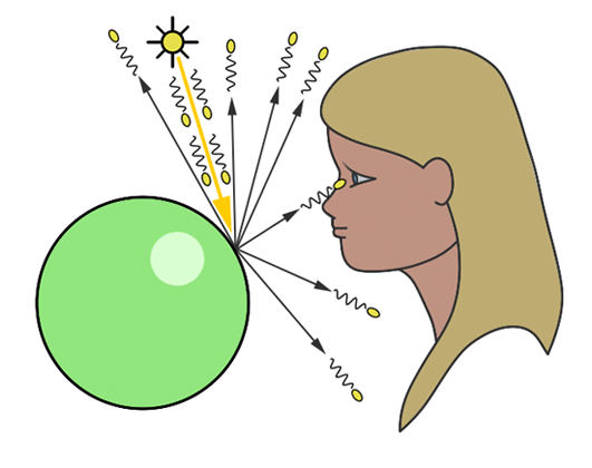
In the image above, countless photons emitted by the light source hit the green sphere, but only one will reach the eye's surface.
Consider the analogy of attempting to paint a teapot by dotting a black sheet of paper with a white marker, with each dot representing a photon. Initially, only a sparse number of photons intersect the teapot, leaving vast areas unmarked. Increasing the dots gradually fills in the gaps, making the teapot progressively more discernible.

However, deploying even thousands or multiples thereof of photons cannot guarantee complete coverage of the object's surface.
This method's inherent flaw necessitates running the program until we subjectively deem enough photons have been applied to accurately depict the object. This process, requiring constant monitoring of the rendering process, is impractical in a production setting. The primary cost in ray tracing lies in detecting ray-geometry intersections, not in generating photons, but in identifying all their intersections within the scene, which is exceedingly resource-intensive.
In summary, Forward ray-tracing or light tracing, which involves casting rays from the light source, can theoretically replicate natural light behavior on a computer. However, as discussed, this technique is neither efficient nor practical for actual use. Let's discuss an alternative apporach:
To make ray tracing more efficient, the method of backward ray-tracing is introduced.
In contrast to the natural process where rays emanate from the light source to the receptor (like our eyes), backward ray-tracing reverses this flow by initiating rays from the receptor towards the objects.
In backward ray-tracing, an eye ray is created at the eye; it passes through the viewplane and on into the world. The first object the eye ray hits is the object that will be visible from that point of the viewplane. After the ray tracer allows that light ray to bounce around, it figures out the exact coloring and shading of that point in the viewplane and displays it on the corresponding pixel on the computer monitor screen.
Upon impacting an object, we evaluate the light it receives by dispatching another ray—termed a light or shadow ray—from the contact point towards the light source. If this "light ray" encounters obstruction by another object, it indicates that the initial point of contact is shadowed, receiving no light. Hence, these rays are more aptly called shadow rays. The inaugural ray shot from the eye (or camera) into the scene is referred to in computer graphics literature as a primary ray, visibility ray, or camera ray.
Backward ray-tracing is also known as eye tracing.
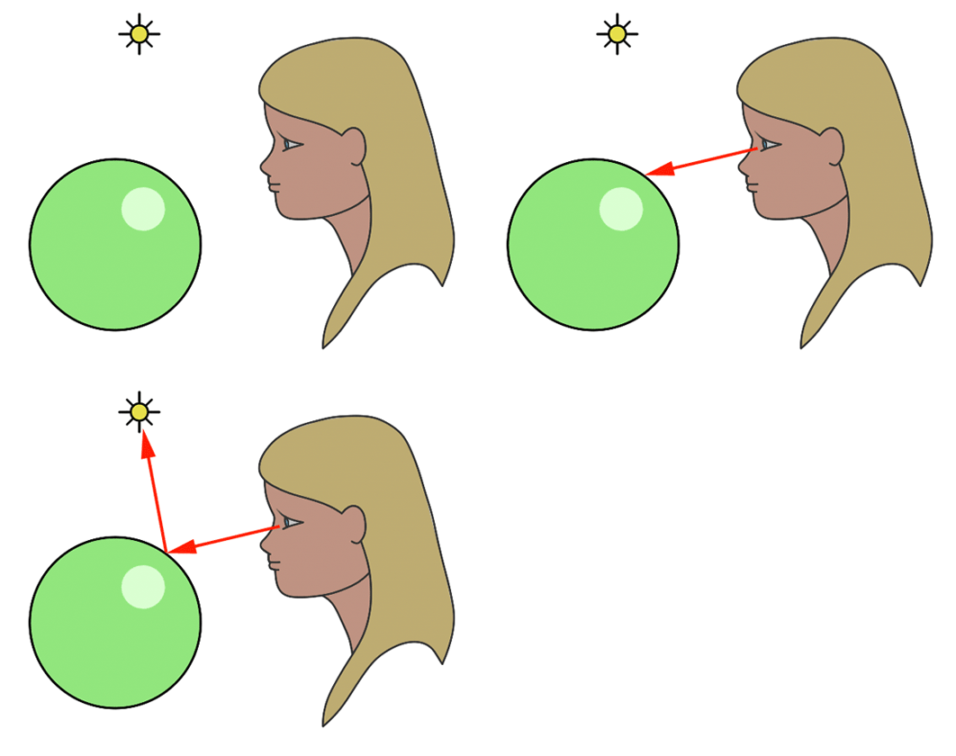
In the image above, we trace a ray from the eye to a point on the sphere, then a ray from that point to the light source.
The downfall of backward ray tracing is that it assumes only the light rays that come through the viewplane and on into the eye contribute to the final image of the scene. In certain cases, this assumption is flawed.
For example, if a lens is held at a distance on top of a table, and is illuminated by a light source directly above, there will exist a focal point beneath the lens with a large concentration of light. If backward ray tracing tries to re-create this image, it will miscalculate because shooting light rays backward only confirms that rays traveled through the lens; backward rays have no way of recognizing that forward rays are bent when they go through the lens.
Therefore, if only backward ray tracing is performed, there will only be an even patch of light beneath the lens, just as if the lens were a normal piece of glass and light is transmitted straight through it.
The technique of initiating rays either from the light source or from the eye is encapsulated by the term path tracing in computer graphics.
While ray-tracing is a synonymous term, path tracing emphasizes the methodological essence of generating computer-generated imagery by tracing the journey of light from its source to the camera, or vice versa. This approach facilitates the realistic simulation of optical phenomena such as caustics or indirect illumination, where light reflects off surfaces within the scene.
The essence of the ray-tracing algorithm is to render an image pixel by pixel.
For each pixel, it launches a primary ray into the scene, its direction determined by drawing a line from the eye through the pixel's center.
This primary ray's journey is then tracked to ascertain if it intersects with any scene objects. In scenarios where multiple intersections occur, the algorithm selects the intersection nearest to the eye for further processing.
A secondary ray, known as a shadow ray, is then projected from this nearest intersection point towards the light source as shown in the following figure:
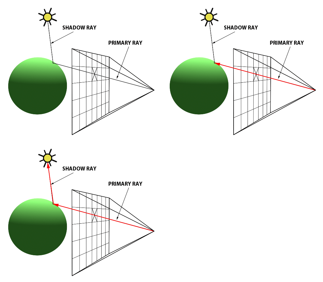
In the image above, a primary ray is cast through the pixel center to detect object intersections. Upon finding one, a shadow ray is dispatched to determine the illumination status of the point.
An intersection point is deemed illuminated if the shadow ray reaches the light source unobstructed. Conversely, if it intersects another object en route, it signifies the casting of a shadow on the initial point.
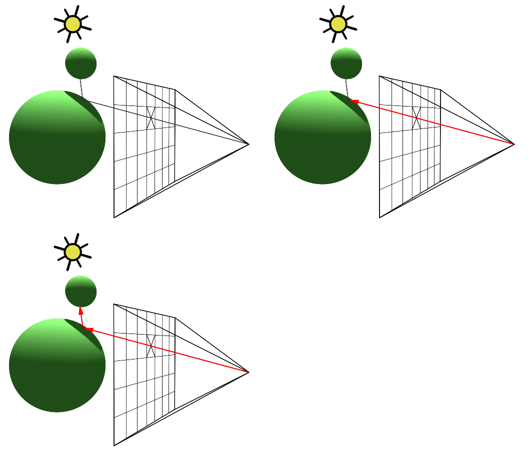
A shadow is cast on the larger sphere by the smaller one, as the shadow ray encounters the smaller sphere before reaching the light.
Repeating this procedure across all pixels yields a two-dimensional depiction of our three-dimensional scene.
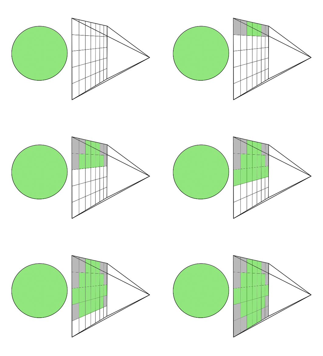
Rendering a frame involves dispatching a primary ray for every pixel within the frame buffer.
The elegance of ray-tracing lies in its simplicity and direct correlation with the physical world, allowing for the creation of a basic ray-tracer in as few as 200 lines of code. This simplicity contrasts sharply with more complex algorithms, like scanline rendering, making ray tracing comparatively effortless to implement.
Regardless of which global lighting model chosen, global lighting models are very expensive to compute. According to Tony DeRose, rendering a single frame of the Pixar movie Finding Nemo took four hours. For The Incredibles, the next Pixar movie, rendering each frame took ten hours, which means that the algorithms have gotten more expensive even though the hardware is speeding up.
Three.js manages to fall somewhere in between, because (as we have already seen) it can use the Scene Graph data structure to compute shadows, but it doesn't do the full ray-tracing or radiosity computation.
Another key benefit of ray-tracing is its capacity to seamlessly simulate intricate optical effects such as reflection and refraction.These capabilities are crucial for accurately rendering materials like glass or mirrored surfaces.
First, let's talk about reflection. Surfaces like metal and glass exhibit a high degree of reflectivity, causing them to mirror their surroundings. This effect is particularly pronounced in materials such as polished metals and glass, where the surface reflects light in a manner akin to a mirror.
Reflections in Three.js can be accomplished quite easily using a CubeCamera.This is a unique camera that contains six perspective cameras that will display what each camera sees onto any object in which you place it. It fits well on all default three dimensional shapes provided by the core threejs library.
CubeCamera is a special type of camera that captures the scene from six different angles, creating a cube map.This cube map can then be used to create realistic reflections on objects in the scene.
// Create the scene
const scene = new THREE.Scene();
scene.background = new THREE.Color(0x87ceeb); // Set background color
const camera = new THREE.PerspectiveCamera(75, window.innerWidth / window.innerHeight, 0.1, 1000);

// Create a WebGLRenderer
const renderer = new THREE.WebGLRenderer();
renderer.setSize(window.innerWidth, window.innerHeight);
document.body.appendChild(renderer.domElement);

// Add lighting
const ambientLight = new THREE.AmbientLight(0x404040, 1); // Soft white light
scene.add(ambientLight);

const directionalLight = new THREE.DirectionalLight(0xffffff, 1);
directionalLight.position.set(5, 5, 5);
scene.add(directionalLight);

const controls = new THREE.OrbitControls(camera, renderer.domElement);

// Create texture loader
const textureLoader = new THREE.TextureLoader();

// Create a CubeCamera for reflections
const cubeRenderTarget = new THREE.WebGLCubeRenderTarget(128, { //128 is the size of the cube map
  format: THREE.RGBFormat, //the color format of the cube map
  generateMipmaps: true, //generate mipmaps for better quality
  //mipmaps are precomputed textures that are used to improve the quality of the texture when viewed at a distance
  minFilter: THREE.LinearMipmapLinearFilter //filter used to sample the texture when viewed at a distance
});

const near = 0.1;
const far = 100;
const cubeCamera = new THREE.CubeCamera(near, far, cubeRenderTarget);
scene.add(cubeCamera);

// Load a texture for the plane
const planeTexture = textureLoader.load('https://raw.githubusercontent.com/amaraauguste/amaraauguste.github.io/refs/heads/master/courses/CISC3620/textures/checkered_pattern.jpg');

// Plane material
const planeMaterial = new THREE.MeshStandardMaterial({
    map: planeTexture,
    roughness: 1,
    metalness: 0,
});

// Create the plane
const planeGeometry = new THREE.PlaneGeometry(20, 20);
const plane = new THREE.Mesh(planeGeometry, planeMaterial);
plane.rotation.x = -Math.PI / 2;
plane.position.y = 0; // Position it on the ground
plane.receiveShadow = true;
scene.add(plane);

// Sphere material
const sphereMaterial = new THREE.MeshStandardMaterial({
    metalness: 1,
    roughness: 0,
    envMap: cubeRenderTarget.texture
});

// Create the reflective sphere
const sphereGeometry = new THREE.SphereGeometry(2, 32, 32);
const sphere = new THREE.Mesh(sphereGeometry, sphereMaterial);
sphere.position.y = 4; // Position it above the plane
sphere.castShadow = true;
scene.add(sphere);

// Position the camera
camera.position.set(0, 5, 10);
controls.update(); // Update controls

// Animation loop
function animate() {
  requestAnimationFrame(animate);

  // Update the CubeCamera position to match the sphere's position
  cubeCamera.position.copy(sphere.position);
  // Update the CubeCamera to capture the environment
  cubeCamera.update(renderer, scene);

  // Render the scene
  renderer.render(scene, camera);
}

animate();
Now we have a reflective sphere on a checkered plane. The CubeCamera captures the scene from the sphere's perspective and creates a cube map that is used to create realistic reflections on the sphere.
This is a simple way to create reflections on surfaces so that we can have more realistic renderings of our objects such as metals.
Three.js can also do refraction. Refraction occurs when light passes through a transparent or translucent object. A ray of light will be bent as it passes between the inside of the object and the outside. This is what happens when you look at a straw in a glass of water and it looks bent.
The amount of bending depends on the so-called "indices of refraction" of the material outside and the material inside the object. More exactly, it depends on the ratio between the two indices. Even a perfectly transparent object will be visible because of the distortion induced by this bending (unless the ratio is 1, meaning that there is no bending of light at all).
In Three.js, refraction is implemented using environment maps.
As with reflection, a refracting object does not show its actual environment; it refracts the cubemap texture that is used as the environment map. For refraction, a special "mapping" must be used for the environment map texture.
The mapping property of a texture tells how that texture will be mapped to a surface. For a cubemap texture being used for refraction, our CubeRenderTargets texture.mapping should be set to THREE.CubeRefractionMapping. (The default value of this property in a cubemap texture is appropriate for reflection rather than refraction.)
And we need to add the refractionRatio property to our sphereMaterial.
So let's start by adjusting out CubeCamera and CubeRenderTargets:
// CubeCamera target
const cubeRenderTarget = new THREE.WebGLCubeRenderTarget(128, {
    format: THREE.RGBFormat,
    generateMipmaps: true,
    minFilter: THREE.LinearMipmapLinearFilter
});

// IMPORTANT TO SET REFRACTION
cubeRenderTarget.texture.mapping = THREE.CubeRefractionMapping;

// Set the near and far for the cubeCamera
const near = 0.1;
const far = 100;
const cubeCamera = new THREE.CubeCamera(near, far, cubeRenderTarget);
scene.add(cubeCamera);
And adjust our sphere properties:
// Sphere
const sphereGeometry = new THREE.SphereGeometry(2, 32, 32);
const sphereMaterial = new THREE.MeshPhongMaterial({
    shininess: 100, //high shininess for a shiny surface
    color: "white", //white color
    specular: "white", //white specular color
    envMap: cubeRenderTarget.texture, //the environment map texture
    refractionRatio: 0.5, //the ratio of the indices of refraction
    transparent: true, //enable transparency
    side: THREE.BackSide, //the side of the object to render
    combine: THREE.MixOperation //mix the environment map with the color of the object
});
const sphere = new THREE.Mesh(sphereGeometry, sphereMaterial);
sphere.position.y = 4; // Slightly above the plane
scene.add(sphere);
We can also now add a GUI to adjust our refraction ratio to see how that changes the effect on the sphere:
// GUI to adjust refraction ratio
const gui = new dat.GUI();
const guiParams = { refractionRatio: sphereMaterial.refractionRatio };

const refractionFolder = gui.addFolder("Refraction");
refractionFolder.add(guiParams, "refractionRatio", 0, 1, 0.01).onChange((v) => {
    sphereMaterial.refractionRatio = v;
});
refractionFolder.open();
And lastly remember to update our cubeCamera in our animate() function:
// Animate function
function animate() {
  requestAnimationFrame(animate);

  // Update cube camera position to match the position of the sphere
  cubeCamera.position.copy(sphere.position);

  // Update cube camera to capture the environment
  cubeCamera.update(renderer, scene);

  // Render scene
  renderer.render(scene, camera);
}
Now we should be able to see the plane refracted through the "glass sphere".
How do the two examples differ? Reflection vs refraction?
Reflection is the bouncing of light off a surface, while refraction is the bending of light as it passes through a medium. In the case of the reflective sphere, the light is bouncing off the surface and creating a mirror-like effect. In the case of the refractive sphere, the light is bending as it passes through the glass and creating a distorted effect.
The important thing to remember is that in the law of (specular) reflection, angle of incidence is equal to the angle of reflection.
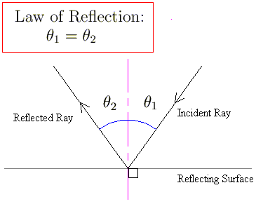
This is similar to what happens to a tennis ball when it hits the surface of the floor. It bounces back in a direction that is symmetrical to the incident direction about the surface normal at the point of impact.
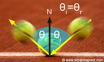
In the image above, the angle of incidence is equal to the angle of reflection.
Computing the reflection direction can be done using simple geometry.
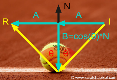
As you can see in image above, the vectors I and R can be expressed in terms of the vectors A and B:
The vector B can easily be computed. It is the projection of the vector I or R onto the vector N. We can compute this vector using the following equation:
As the term cos(θ) is equal to the dot product between the two vectors N and I.
We can now replace B in both equations:
And we can re-write the first equation as follows:
We can now compute the vector R as:
A reflection of a light ray can only be seen if the reflected ray direction is traveling in the same direction as the view direction.
The fact that the reflected image of the objects in the scene from which these light rays are emitted changes with the view direction is the reason why we say that reflection is view-dependent.
If you look at the reflection of a static object in the mirror and change direction, you will see that the image of that object changes. This is something that we find natural when we look at an object from a different angle, but that we find maybe less natural when we change our position with respect to a mirror reflecting that same object, though the reason why this is happening is essentially the same. We look at a different part of the object.
By opposition, we say that diffuse reflections are view independent because they don't vary with the angle of view.
Note that the reflection process is potentially recursive. It is entirely possible to have a situation in which a ray intersects a reflective surface from which we cast another reflection ray, that will intersect in turn another reflective surface, etc. In other words, the process will keep casting reflection rays unless the ray intersects an object which is not a mirror or if it doesn't intersect anything at all (in which case we return the background color).
If a ray kept reflecting other reflecting surfaces without ever reflecting anything else, we would then enter some kind of infinite recursive process. To prevent this from happening, we generally put a cap or limit on the number of recursions.
The number of times a reflection ray is reflected off of surfaces is called the ray depth. When we cast a reflection ray from the primary ray, we say that the ray has a depth of 1. After two reflections, the ray has a depth of 2, and so on.
For most scenes using a depth much greater than 4 or 5 generally doesn't make much of a visual difference. It's only when very complex transparent surfaces are rendered (such as water splashes) that using a depth much greater than 5 is necessary for producing images that are similar to the real thing.
Keep in mind that another reason for putting a cap on the recursion depth is also because ray-tracing is expensive. The higher the recursion the longer it will take to render a frame.
In the case of refraction, the angle of incidence is not equal to the angle of refraction. The amount of bending depends on the index of refraction (ior).
The index of refraction for glass and water is around 1.5 and 1.3 respectively. For a fixed angle of incidence, the amount of bending depends on the index of refraction (as shown in the image below):
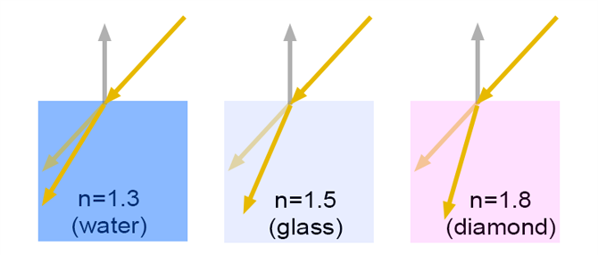
Refraction is described by Snell's law, which states that for a given pair of media, the ratio of the sines of the angle of incidence and angle of refraction is equivalent to the opposite ratio of the indices of refraction.
Snell's Law:
Let's look at them side by side: here
Notice how both spheres either reflect or refract the environment around them.
The problem with this image though, is that it is not completely realistic. Glass spheres as well as pretty much every other transparent surface (water, diamonds, crystals, etc.) transmit as well as reflect light. They are both refractive and reflective (not either or). The problem is how do we know how much light they transmit vs. the amount of light they reflect?
This ratio is given by the Fresnel equations.
Transparent objects such as glass or water are both refractive and reflective. How much light they reflect vs the amount they transmit depends on the angle of incidence. The amount of transmitted light increases when the angle of incidence decreases.
And since by the principle of the conservation of energy, the amount of reflected light plus the amount of refracted light is necessarily equal to the total amount of incident light, you can deduce that the amount of reflected light increases when the angle of incidence increases, up to 100% as the angle gets closer to 90 degrees.
Technically, the edges of a glass ball are 100% reflective. In its center though, the sphere only reflects about 6% of the incident light.
The amount of reflected vs. refracted light can be computed using what we call the Fresnel equations. Explaining the origin of these equations and how they can be derived goes far beyond the level of explanation we are willing to give in this lesson.
Light is composed of two perpendicular waves which we call parallel and perpendicular polarised light. Don't worry too much if you don't know about this detail.
Suffice it to know that we need to compute the ratio of reflected light for these two waves using two different equations (one for each type of wave) and average the results to find the solution.
The two Fresnel equations are:
By taking the average of the two we get the actual ratio of reflected light:
The terms , are the refraction indices of the two mediums. The terms and are the angles of incidence and refraction respectively. As mentioned before, due to the conservation of energy, the ratio of refracted light can simply be computed as:
Keep in mind that if the light goes from one medium to another medium with a lower refraction index, it may be subject to the phenomenon of total internal reflection. This is happening in the case of materials such as glass or water, so we need to take this into account.
We do so by computing as in the case of reflection, the sine of the angle of refraction or . If is greater than 1, then we have a case of total reflection. In this particular case, there is no need to compute the Fresnels formulas, we can just set to 1.
As usual, you will need to swap the refraction indices if you find out that the incident ray is inside the object with the greatest refraction index. This can be done again by testing the sign of the cosine of the angle between the surface normal and the incident ray direction (the sign of ).
The fresnel effect can easily be observed in nature.
If you look at the picture of the lake with some mountains in the background and pebbles in the foreground, you can see that the reflection seems to increase with distance.
Note also that while reflections are strong in the distance, we see more clearly through the water in the foreground than we do in the far distance. This is due to fresnel.
The angle of incidence increases with the distance as shown in the following image:
and we know that the ratio of reflection vs. transmission increases with the angle of incidence. Thus naturally as we look in the distance, the water's surface reflects more light.
Though if we look almost directly down on the water surface, a few meters from where we stand, the angle incidence is low and most of the light is transmitted. Thus we see through the water more clearly than when we look in the distance.
You can easily observe this effect on a large variety of objects: the facade of a building made out of glass, glass balls that are more reflective on the edges, etc.
But back to our example, we can see that the CubeCamera is a very useful tool for creating realistic reflections and refractions in our scenes.
CubeCamera can take a six-fold picture of a scene from a given point of view and make a cubemap texture from those images. To use the camera, we have to place it at the location of an object—and make the object invisible so it doesn't show up in the pictures. Snap the picture, and apply it as an environment map on the object.
For animated scenes, you have to do this in every frame, and we need to do it for every reflective/refractive object in the scene. Obviously, this can get very computationally expensive! And the result still isn't perfect.
There is also the case where we do not want to use the exact environment around our object but instead use a different environment. This is where we can use a CubeTextureLoader to load a cubemap texture (opposed to capturing our current environment with a CubeCamera) from a set of images.
We have created and viewed simple scenes, shown on a solid-colored background, but it would be nice to put our scenes in an "environment" such as the interior of a building, a nature scene, or a public square.
It's not practical to build representations of such complex environments out of geometric primitives, but we can get a reasonably good effect using textures.
The technique that is used in Three.js is called a skybox.
A skybox is a large cube — effectively, infinitely large — where a different texture is applied to each face of the cube. The textures are images of some environment. For a viewer inside the cube, the six texture images on the cube fit together to provide a complete view of the environment in every direction.
The six texture images together make up what is called a cubemap texture. The images must match up along the edges of the cube to form a seamless view of the environment.
A cube map of an actual physical environment can be made by taking six pictures of the environment in six directions: left, right, up, down, forward, and back. (More realistically, it is made by taking enough photographs to cover all directions, with overlaps, and then using software to "stitch" the images together into a complete cube map.)
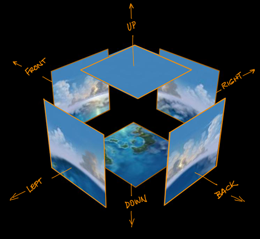
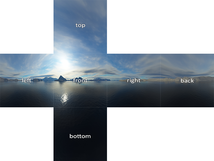
The six directions are referred to by their relation to the coordinate axes as: positive x, negative x, positive y, negative y, positive z, and negative z, and the images must be listed in that order when you specify the cube map.
Here is an example - The first picture shows the six images of a cube map laid out next to each other.
The positive y image is at the top, the negative y image is at the bottom. In between are the negative x, positive z, positive x, and negative z images laid out in a row.
The second picture shows the images used to texture a cube, viewed here from the outside. You can see how the images match up along the edges of the cube:
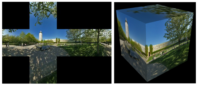
For a skybox, conceptually, a very large cube would be used. The camera, lights, and any objects that are to be part of the scene would be inside the cube. It is possible to construct a skybox by hand in just this way.
Let's create a cubemap/skybox contained within a cube:
//creating a cube
const geometry = new THREE.BoxGeometry(8,8,8);
var materials = [
    new THREE.MeshBasicMaterial({
        map : new THREE.TextureLoader().load('https://raw.githubusercontent.com/amaraauguste/amaraauguste.github.io/refs/heads/master/courses/CISC3620/textures/Daylight%20Box_Pieces/Daylight%20Box_PosX.bmp'),
        side : THREE.BackSide,
    }),
    new THREE.MeshBasicMaterial({
        map : new THREE.TextureLoader().load('https://raw.githubusercontent.com/amaraauguste/amaraauguste.github.io/refs/heads/master/courses/CISC3620/textures/Daylight%20Box_Pieces/Daylight%20Box_NegX.bmp'),
        side : THREE.BackSide,
    }),
    new THREE.MeshBasicMaterial({
        map : new THREE.TextureLoader().load('https://raw.githubusercontent.com/amaraauguste/amaraauguste.github.io/refs/heads/master/courses/CISC3620/textures/Daylight%20Box_Pieces/Daylight%20Box_PosY.bmp'),
        side : THREE.BackSide,
    }),
    new THREE.MeshBasicMaterial({
        map : new THREE.TextureLoader().load('https://raw.githubusercontent.com/amaraauguste/amaraauguste.github.io/refs/heads/master/courses/CISC3620/textures/Daylight%20Box_Pieces/Daylight%20Box_NegY.bmp'),
        side : THREE.BackSide,
    }),
    new THREE.MeshBasicMaterial({
        map : new THREE.TextureLoader().load('https://raw.githubusercontent.com/amaraauguste/amaraauguste.github.io/refs/heads/master/courses/CISC3620/textures/Daylight%20Box_Pieces/Daylight%20Box_PosZ.bmp'),
        side : THREE.BackSide,
    }),
    new THREE.MeshBasicMaterial({
        map : new THREE.TextureLoader().load('https://raw.githubusercontent.com/amaraauguste/amaraauguste.github.io/refs/heads/master/courses/CISC3620/textures/Daylight%20Box_Pieces/Daylight%20Box_NegZ.bmp'),
        side : THREE.BackSide,
    }),
];
const cube = new THREE.Mesh(geometry,materials);
scene.add(cube);

camera.position.set(0, 0, 15);
Based on this we should see a cube with the six images of the cube map applied inside it.
However, Three.js makes it very easy to use a skybox as the background for a scene. It has the class THREE.CubeTexture to represent cube maps, and you can enclose your scene in a skybox simply by assigning a CubeTexture as the value of the property scene.background. (The value of that property could also be a normal Texture or a Color.)
A CubeTexture can be created by a CubeTextureLoader, which can load the six images that make up the cube map. The loader has a method named load() that works in the same way as the load() method of a TextureLoader, except that the first parameter to the method is an array of six strings giving the URLs of the six images for the cube map.
Now, let's load a texture map for a meadow (this particular cube map, and others like it, are by Emil Persson, who has made a large number of cube maps available for download at http://www.humus.name/index.php?page=Textures under a creative commons license or from sources like opengameart.org which is where the previous textures came from).
const textureURLs = [  // URLs of the six faces of the cube map (in the order: +x, -x, +y, -y, +z, -z)
    "https://raw.githubusercontent.com/amaraauguste/amaraauguste.github.io/refs/heads/master/courses/CISC3620/textures/Meadow/posx.jpg",
    "https://raw.githubusercontent.com/amaraauguste/amaraauguste.github.io/refs/heads/master/courses/CISC3620/textures/Meadow/negx.jpg",
    "https://raw.githubusercontent.com/amaraauguste/amaraauguste.github.io/refs/heads/master/courses/CISC3620/textures/Meadow/posy.jpg",
    "https://raw.githubusercontent.com/amaraauguste/amaraauguste.github.io/refs/heads/master/courses/CISC3620/textures/Meadow/negy.jpg",
    "https://raw.githubusercontent.com/amaraauguste/amaraauguste.github.io/refs/heads/master/courses/CISC3620/textures/Meadow/posz.jpg",
    "https://raw.githubusercontent.com/amaraauguste/amaraauguste.github.io/refs/heads/master/courses/CISC3620/textures/Meadow/negz.jpg"
];
const cubeLoader = new THREE.CubeTextureLoader();
const cubeTexture = cubeLoader.load(textureURLs);
scene.background = cubeTexture;
Now we should see our environment as our scene is now surrounded by the skybox texture.
Let's put our reflective sphere into this environment and see how it works:
// Create a cube render target for reflections
const cubeRenderTarget = new THREE.WebGLCubeRenderTarget(128, {
    format: THREE.RGBFormat,
    generateMipmaps: true,
    minFilter: THREE.LinearMipmapLinearFilter
});

const near = 0.1;
const far = 100;
const cubeCamera = new THREE.CubeCamera(near, far, cubeRenderTarget);
scene.add(cubeCamera);

// Sphere for reflection
const sphereReflectionMaterial = new THREE.MeshStandardMaterial({
    metalness: 1,
    roughness: 0,
    envMap: cubeRenderTarget.texture
});
const sphereReflection = new THREE.Mesh(
    new THREE.SphereGeometry(50, 32, 32),
    sphereReflectionMaterial
);
sphereReflection.position.y = 4;
sphereReflection.position.x = -53; // Position it on the left
scene.add(sphereReflection);
And remember to add the following to our animate() function:
// Update cube camera for reflection
cubeCamera.position.copy(sphereReflection.position);
cubeCamera.update(renderer, scene);
What effect does the skybox have on the reflective sphere?
The skybox provides a background environment for the reflective sphere, allowing it to reflect the surrounding scenery. The reflections on the sphere will now show the meadow environment instead of a solid color.
Let's add our refractive sphere too:
// Create a cube render target for refractions
const cubeRenderTarget2 = new THREE.WebGLCubeRenderTarget(128, {
  format: THREE.RGBFormat,
  generateMipmaps: true,
  minFilter: THREE.LinearMipmapLinearFilter
});

const cubeCamera2 = new THREE.CubeCamera(near, far, cubeRenderTarget2);
scene.add(cubeCamera2);

// Important to set for refraction
cubeRenderTarget2.texture.mapping = THREE.CubeRefractionMapping;

// Sphere for refraction
const sphereRefractionMaterial = new THREE.MeshPhongMaterial({
    shininess: 100,
    color: 0xffffff,
    specular: 0xffffff,
    envMap: cubeRenderTarget2.texture,
    refractionRatio: 0.5,
    transparent: true,
    side: THREE.BackSide // Render from inside
});
const sphereRefraction = new THREE.Mesh(
    new THREE.SphereGeometry(50, 32, 32),
    sphereRefractionMaterial
);
sphereRefraction.position.y = 4;
sphereRefraction.position.x = 53; // Position it on the right
scene.add(sphereRefraction);
And once again update in our animate() function:
// Update cube camera for refraction
cubeCamera2.position.copy(sphereRefraction.position);
cubeCamera2.update(renderer, scene);
Now we should have a sphere for reflecting and a sphere for refracting the cubemap environment around them.
Ray casting (or Object Picking) is the process in a ray-tracing algorithm that shoots one or more rays from the camera (eye position) through each pixel in an image plane, and then tests to see if the rays intersect any primitives (triangles) in the scene. If a ray passing through a pixel and out into the 3D scene hits a primitive, then the distance along the ray from the origin (camera or eye point) to the primitive is determined, and the color data from the primitive contributes to the final color of the pixel. The ray may also bounce and hit other objects and pick up color and lighting information from them.
Ray casting is critical for rendering and visualization because it creates realistic lighting. This technique simulates how light interacts with objects in the real world in a digital environment, which allows for astonishingly realistic characters, objects, and scenes.
Ray casting is a fundamental technique for modern 3D design, but the technology is decades old. In the 1960s, computer scientists explored methods to simulate how light interacts with surfaces for realistic image generation. In the 1980s, Turner Whitted wrote a paper on recursive ray tracing that popularized the technique. It introduced the concept of handling reflections and refractions by recursively casting rays — a true game-changer for ray casting.
John Carmack popularized ray casting in the early 1990s with the game "Wolfenstein 3D", which used ray casting to create a 3D perspective in a 2D world. In the 2000s, ray casting techniques blended with rasterization to support real-time rendering in digital simulations. Today, companies are developing hardware-accelerated ray tracing, which pushes the boundaries of what's possible.
Ray casting has many important applications, such as:
We can use ray casting as a way to determine where the user's mouse is pointing in a 3D scene.
Essentially, a pointer is cast from your mouse or finger (on mobile) through the frustum (the shape of the region that can be seen and rendered by a perspective camera) of the scene to the object that it intersects.
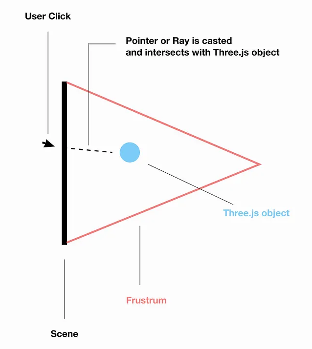
In Three.js, ray casting can be achieved using Vector2D and the Raycaster.
The Raycaster is given the coordinates of the mouse on the screen, and it creates a ray normal to the mouse's position.This allows the Raycaster to determine the objects that the ray is intersecting using the intersectObjects method.
A Raycaster takes an initial point and a direction, given as a vector. The point and vector determine a ray, that is, a half-infinite line that extends from a starting point, in some direction, to infinity.
The Raycaster can find all the intersections of the ray with a given set of objects in a three.js scene, sorted by order of distance from the rays's starting point.
The syntax for using the Raycaster is as follows:
const raycaster = new THREE.Raycaster();To tell it which ray to use, you can call:
raycaster.set(startingPoint, direction);or more specifically set from camera:
raycaster.setFromCamera(mouse, camera);Here, along with the Raycaster, we also need to initialize a Vector2 that will hold the coordinates of the mouse.
A Vector2 is a two-dimensional vector that only contains the x and y coordinates. We use this to track the movement of the cursor on the screen.
The syntax for creating a Vector2 is as follows:
const mouse = new THREE.Vector2();To set the coordinates of the mouse, we can use the following syntax:
mouse.set(x, y);Where x and y are the coordinates of the mouse on the screen.
To get the coordinates of the mouse, we can use the following syntax:
mouse.x = (event.clientX / width) * 2 - 1;And
mouse.y = -(event.clientY / height) * 2 + 1;Where event is the event object that is passed to the event handler.
We multiply by 2 and subtract 1 to get the coordinates in the range of -1 to 1.
We also need to set the camera to the Raycaster. The camera is the point of view from which we are looking at the scene.
To check if the ray intersects with any objects in the scene, we can use the following syntax:
const intersects = raycaster.intersectObjects(objects);Where objects is an array of objects in the scene.
Let's try an example:
const width = 500;
const height = 400;

const scene = new THREE.Scene();
const camera = new THREE.PerspectiveCamera(75, width / height, 0.1, 1000);

const renderer = new THREE.WebGLRenderer();
renderer.setSize(width, height);
document.body.appendChild(renderer.domElement);

// Position the camera
camera.position.set(0, 0, 10);

// Lights
const hemisphere = new THREE.HemisphereLight("white", "gray", 1);
scene.add(hemisphere);
const directional = new THREE.DirectionalLight("white", 0.5);
directional.position.set(5, 5, 5);
scene.add(directional);

// Objects array for raycasting
const objects = [];

// Geometry
const geometry = new THREE.SphereGeometry(3, 64, 64);
// Material
const material = new THREE.MeshStandardMaterial({
  color: "red",
  metalness: 0.5,
  roughness: 1
});
// Mesh
const circle = new THREE.Mesh(geometry, material);
scene.add(circle);
objects.push(circle); // Store the circle in the objects array

// Mouse event for color change
document.addEventListener("mousedown", onMouseDown);
function onMouseDown(event) {
  event.preventDefault();
  const mouse = new THREE.Vector2();
  mouse.set((event.clientX / width) * 2 - 1, -(event.clientY / height) * 2 + 1);
  const raycaster = new THREE.Raycaster();
  raycaster.setFromCamera(mouse, camera);
  const intersects = raycaster.intersectObjects(objects);
  if (intersects.length > 0) { // Check if there is an intersection
    // Change the color of the intersected object
    intersects[0].object.material.color.setHex(Math.random() * 0xffffff);
  }
}

// Animation loop
function animate() {
  requestAnimationFrame(animate);

  // Render the scene from the perspective of the camera
  renderer.render(scene, camera);
}

animate();
In this example, we create a scene with a red sphere. When the user clicks on the sphere, it changes color to a random color.
We use the Raycaster to check if the mouse intersects with the sphere. If it does, we change the color of the sphere.
We can also use the Raycaster to check if the mouse intersects with other objects in the scene.
For example, we can create a plane and check if the mouse intersects with it:
const planeGeometry = new THREE.PlaneGeometry(20, 20);
const planeMaterial = new THREE.MeshStandardMaterial({ color: "blue", side: THREE.DoubleSide });
const plane = new THREE.Mesh(planeGeometry, planeMaterial);
plane.rotation.x = -Math.PI / 2; // Rotate the plane to be horizontal
plane.position.y = -2.75; // Position the plane below the sphere
scene.add(plane);
objects.push(plane); // Store the plane in the objects array
Now, when the user clicks on the plane, it will also change color to a random color.
Let's use the Raycaster to create a scene with more functionality.
The scene shows a square, green base, and some tapered, yellow cylinders standing on the base. Cylinders can intersect; no attempt is made to treat them like real solid objects.
The user can interact with the scene using the mouse.
Three radio buttons let the user select the action that they want to perform with the mouse.
const width = 500;
const height = 400;

// Create the scene and camera
const scene = new THREE.Scene();
const camera = new THREE.PerspectiveCamera(75, width / height, 0.1, 1000);
camera.position.set(-30, 40, 10);
camera.lookAt(0, 0, 0);

// Create the renderer
const renderer = new THREE.WebGLRenderer();
renderer.setSize(width, height);
document.body.appendChild(renderer.domElement);

// Add lights
const directionalLight = new THREE.DirectionalLight(0xffffff, 1);
directionalLight.position.set(5, 10, 7.5);
scene.add(directionalLight);

const ambientLight = new THREE.AmbientLight(0x404040); // Soft white light
scene.add(ambientLight);

// Create ground
const ground = new THREE.Mesh(
  new THREE.BoxGeometry(40, 1, 40),
  new THREE.MeshLambertMaterial({ color: "green" })
);
ground.position.y = -0.5;
scene.add(ground);

// Create variables for interactivity
const raycaster = new THREE.Raycaster();
const mouse = new THREE.Vector2();
let mouseAction = 1; // Default to ADD = 1
let dragItem = null; // To track the object being dragged

// Functions for interaction
function addCylinder(x, z) {
  const cylinderGeometry = new THREE.CylinderGeometry(1, 2, 6, 16, 1);
  const cylinderMaterial = new THREE.MeshLambertMaterial({ color: "yellow" });
  const cylinder = new THREE.Mesh(cylinderGeometry, cylinderMaterial);
  cylinder.position.set(x, 3, z);
  scene.add(cylinder);
}

function handleMouseDown(event) {
  mouse.x = (event.clientX / width) * 2 - 1;
  mouse.y = -(event.clientY / height) * 2 + 1;
  raycaster.setFromCamera(mouse, camera);

  const intersects = raycaster.intersectObjects(scene.children);
  if (intersects.length > 0) {
    const objectHit = intersects[0].object;

    // Only interact with the ground or cylinders
    if (mouseAction === 1) {
      // ADD
      const coords = intersects[0].point;
      addCylinder(coords.x, coords.z);
    } else if (mouseAction === 2) {
      // DRAG
      // Only start dragging if the item is not the ground
      if (objectHit !== ground) {
        dragItem = objectHit;
      }
    } else if (mouseAction === 3) {
      // DELETE
      // Check if the clicked object is NOT the ground
      if (objectHit !== ground) {
        scene.remove(objectHit);
      }
    }
  }
}

function handleMouseMove(event) {
  if (!dragItem) return; // Only proceed if an item is being dragged
  mouse.x = (event.clientX / width) * 2 - 1;
  mouse.y = -(event.clientY / height) * 2 + 1;
  raycaster.setFromCamera(mouse, camera);

  const intersects = raycaster.intersectObject(ground);
  if (intersects.length > 0) {
    // Use the intersection point to set the position of the dragItem.
    // Ensure dragItem's scale is untouched; it should remain the same as originally created.
    dragItem.position.copy(intersects[0].point);
    dragItem.position.y = 3; // Keep the cylinder at a fixed height
  }
}

function handleMouseUp() {
  dragItem = null; // Release the dragged item
}

function doChangeMouseAction() {
  const checkedAction = document.querySelector(
    'input[name="mouseAction"]:checked'
  );
  if (checkedAction) {
    switch (checkedAction.id) {
      case "mouseAdd":
        mouseAction = 1;
        break;
      case "mouseDrag":
        mouseAction = 2;
        break;
      case "mouseDelete":
        mouseAction = 3;
        break;
    }
  }
}

// Event listeners
window.addEventListener("mousedown", handleMouseDown);
window.addEventListener("mousemove", handleMouseMove);
window.addEventListener("mouseup", handleMouseUp);

// Animation loop
function animate() {
  requestAnimationFrame(animate);
  renderer.render(scene, camera);
}
animate();
Now we have a scene where we can add, drag, and delete cylinders using the mouse.
Particle effects are a way to simulate and render large numbers of small, simple objects in a scene.
They are often used to create effects like smoke, fire, rain, snow, and explosions.
In Three.js, particle effects can be created using the THREE.Points class.
The THREE.Points class is a type of geometry that represents a collection of points in 3D space.
Each point can have its own color, size, and other properties.
To create a particle effect, we can create a geometry and a material, and then use the THREE.Points class to create a mesh.
For example, we can create a particle effect that simulates falling confetti:
const particleCount = 1000;
const particles = new THREE.BufferGeometry();
const positions = new Float32Array(particleCount * 3); // 3 coordinates for each particle
const colors = new Float32Array(particleCount * 3); // 3 color values for each particle

const sizes = new Float32Array(particleCount); // Size for each particle

for (let i = 0; i < particleCount; i++) {
  // Random position
  positions[i * 3] = (Math.random() - 0.5) * 100; // x
  positions[i * 3 + 1] = (Math.random() - 0.5) * 100; // y
  positions[i * 3 + 2] = (Math.random() - 0.5) * 100; // z

  // Random color
  colors[i * 3] = Math.random(); // r
  colors[i * 3 + 1] = Math.random(); // g
  colors[i * 3 + 2] = Math.random(); // b

  // Random size
  sizes[i] = Math.random() * 5; // Size between 0 and 5

}

particles.setAttribute("position", new THREE.BufferAttribute(positions, 3));
particles.setAttribute("color", new THREE.BufferAttribute(colors, 3)); // Set color attribute

particles.setAttribute("size", new THREE.BufferAttribute(sizes, 1)); // Set size attribute

const particleMaterial = new THREE.PointsMaterial({
    size: 1,
    vertexColors: true, // Use vertex colors
    sizeAttenuation: true, // Size decreases with distance
    transparent: true,
    opacity: 0.5,
});


const particleSystem = new THREE.Points(particles, particleMaterial);

scene.add(particleSystem);
In this example, we create a particle system with 1000 particles.
Each particle has a random position, color, and size.
We use the THREE.BufferGeometry class to create a geometry that can hold a large number of points.
We set the position, color, and size attributes of the geometry using the setAttribute method.
We create a material using the THREE.PointsMaterial class, which allows us to set the size and color of the particles.
Finally, we create a THREE.Points object using the geometry and material, and add it to the scene.
We can also animate the particles to create a falling confetti effect:
function animateParticles() {
    const positionArray = particles.attributes.position.array;

    // Update the positions of the particles to create a falling effect
    for (let i = 0; i < particleCount; i++) {
        positionArray[i * 3 + 1] -= 0.1; // Move down
        if (positionArray[i * 3 + 1] < -50) {
            positionArray[i * 3 + 1] = 50; // Reset to the top
        }
    }

    particles.attributes.position.needsUpdate = true; // Mark the position attribute as needing an update
}

function animate() {
    requestAnimationFrame(animate);
    renderer.render(scene, camera);
    animateParticles(); // Call the particle animation function
}
animate();
In this example, we update the y-coordinate of each particle to create a falling effect.
When a particle goes below a certain threshold, we reset its position to the top of the screen.
We also rotate the particle system to create a nice effect.
We can also create other particle effects, such as fire, smoke, and explosions, using the same technique.
For example, we can create a fire effect using a particle system with a red-orange color and a larger size.
We can also use textures to create more complex particle effects.
For example, we can use a texture of a snowflake to create a snow effect:
const snowflakeTexture = new THREE.TextureLoader().load("https://raw.githubusercontent.com/amaraauguste/amaraauguste.github.io/refs/heads/master/courses/CISC3620/textures/snowflake.png");
const particleMaterial = new THREE.PointsMaterial({
  size: 1,
  alphaTest: 0.25, // Discard pixels with an alpha value below this threshold so we don't see the edges of the texture
  map: snowflakeTexture, // Use the snowflake texture
  transparent: true,
  sizeAttenuation: true, // Size decreases with distance
  vertexColors: true, // Use vertex colors
  opacity: 0.5,
});
Now we should see randomly colored snowflakes falling from the sky.
To make these snowflakes one color (e.g. white) we can modify our colors to have the same value for each particle:
for (let i = 0; i < particleCount; i++) {
  // Random position
  positions[i * 3] = (Math.random() - 0.5) * 100; // x
  positions[i * 3 + 1] = (Math.random() - 0.5) * 100; // y
  positions[i * 3 + 2] = (Math.random() - 0.5) * 100; // z

  // White color
  colors[i * 3] = 1; // r
  colors[i * 3 + 1] = 1; // g
  colors[i * 3 + 2] = 1; // b

  // Random size
  sizes[i] = Math.random() * 5; // Size between 0 and 5
} // Set the color to white for all particles
Now we should see white snowflakes falling from the sky.
Let's contain these snowflakes to a certain area, like within a cube:
First, we have to set our bounding for the snowflakes:
// Size of the cube that contains the snowflakes
const cubeSize = 100; // Size of the cube

for (let i = 0; i < particleCount; i++) {
  // Initialize the snowflakes within the cube
  positions[i * 3] = (Math.random() - 0.5) * cubeSize; // X position
  positions[i * 3 + 1] = Math.random() * cubeSize; // Y position starts from 0 to cubeSize
  positions[i * 3 + 2] = (Math.random() - 0.5) * cubeSize; // Z position

  // Set particle color to white
  colors[i * 3] = 1; // Red
  colors[i * 3 + 1] = 1; // Green
  colors[i * 3 + 2] = 1; // Blue

  sizes[i] = Math.random() * 5;
}
Then we can create a wireframe cube to house our snowflakes
// Create a cube to contain the snowflakes
const cubeGeometry = new THREE.BoxGeometry(cubeSize, cubeSize, cubeSize);
const cubeMaterial = new THREE.LineBasicMaterial({ color: 0x00ff00 }); // Green color for wireframe
const cubeEdges = new THREE.EdgesGeometry(cubeGeometry); // Creates edges for the cube
const cubeWireframe = new THREE.LineSegments(cubeEdges, cubeMaterial);
scene.add(cubeWireframe);
cubeWireframe.position.y = 50;

camera.position.set(0, 50, 150);
Let's use what we know about skyboxes to better contain our snow scene:
const scene = new THREE.Scene();
const camera = new THREE.PerspectiveCamera(75, window.innerWidth / window.innerHeight, 0.1, 1000);
const renderer = new THREE.WebGLRenderer();
renderer.setSize(window.innerWidth, window.innerHeight);
document.body.appendChild(renderer.domElement);

// Add Orbit Controls
const controls = new THREE.OrbitControls(camera, renderer.domElement);

const particleCount = 1000;
const particles = new THREE.BufferGeometry();
const positions = new Float32Array(particleCount * 3);
const colors = new Float32Array(particleCount * 3);
const sizes = new Float32Array(particleCount);

// Size of the cube that contains the snowflakes
const cubeSize = 100;

for (let i = 0; i < particleCount; i++) {
    // Initialize the snowflakes within the cube
    positions[i * 3] = (Math.random() - 0.5) * cubeSize; // X position
    positions[i * 3 + 1] = Math.random() * cubeSize; // Y position starts from 0 to cubeSize
    positions[i * 3 + 2] = (Math.random() - 0.5) * cubeSize; // Z position

    // Set particle color to white
    colors[i * 3] = 1; // Red
    colors[i * 3 + 1] = 1; // Green
    colors[i * 3 + 2] = 1; // Blue

    sizes[i] = Math.random() * 5;
}

// Create a cube to contain the snowflakes
const cubeGeometry = new THREE.BoxGeometry(cubeSize, cubeSize, cubeSize);
var materials = [
  new THREE.MeshBasicMaterial({
    map: new THREE.TextureLoader().load('https://raw.githubusercontent.com/amaraauguste/amaraauguste.github.io/refs/heads/master/courses/CISC3620/textures/winter%20world/frost_posX.png'), side: THREE.BackSide,
  }),
  new THREE.MeshBasicMaterial({
    map: new THREE.TextureLoader().load('https://raw.githubusercontent.com/amaraauguste/amaraauguste.github.io/refs/heads/master/courses/CISC3620/textures/winter%20world/frost_negX.png'), side: THREE.BackSide,
  }),
   new THREE.MeshBasicMaterial({
    map: new THREE.TextureLoader().load('https://raw.githubusercontent.com/amaraauguste/amaraauguste.github.io/refs/heads/master/courses/CISC3620/textures/winter%20world/frost_posY.png'), side: THREE.BackSide,
  }),
   new THREE.MeshBasicMaterial({
    map: new THREE.TextureLoader().load('https://raw.githubusercontent.com/amaraauguste/amaraauguste.github.io/refs/heads/master/courses/CISC3620/textures/winter%20world/frost_negY.png'), side: THREE.BackSide,
  }),
   new THREE.MeshBasicMaterial({
    map: new THREE.TextureLoader().load('https://raw.githubusercontent.com/amaraauguste/amaraauguste.github.io/refs/heads/master/courses/CISC3620/textures/winter%20world/frost_posZ.png'), side: THREE.BackSide,
  }),
   new THREE.MeshBasicMaterial({
    map: new THREE.TextureLoader().load('https://raw.githubusercontent.com/amaraauguste/amaraauguste.github.io/refs/heads/master/courses/CISC3620/textures/winter%20world/frost_negZ.png'), side: THREE.BackSide,
  })
];

const cube = new THREE.Mesh(cubeGeometry,materials);
scene.add(cube);
cube.position.y = 50;

camera.position.set(0, 50, 200);
particles.setAttribute("position", new THREE.BufferAttribute(positions, 3));
particles.setAttribute("color", new THREE.BufferAttribute(colors, 3));
particles.setAttribute("size", new THREE.BufferAttribute(sizes, 1));

const snowflakeTexture = new THREE.TextureLoader().load("https://raw.githubusercontent.com/amaraauguste/amaraauguste.github.io/refs/heads/master/courses/CISC3620/textures/snowflake.png");
const particleMaterial = new THREE.PointsMaterial({
    size: 2,
    alphaTest: 0.25,
    map: snowflakeTexture,
    transparent: true,
    sizeAttenuation: true,
    vertexColors: true,
    opacity: 1,
});

const particleSystem = new THREE.Points(particles, particleMaterial);
scene.add(particleSystem);

function animateParticles() {
    for (let i = 0; i < particleCount; i++) {
        // Move the snowflakes down
        positions[i * 3 + 1] -= 0.1;

        // Check if the snowflake is out of bounds
        if (positions[i * 3 + 1] < 0) {
          // Reset Y position to the top of the cube
          positions[i * 3 + 1] = cubeSize;
          // Randomize X and Z positions within the cube bounds
          positions[i * 3] = (Math.random() - 0.5) * cubeSize; // New X position
          positions[i * 3 + 2] = (Math.random() - 0.5) * cubeSize; // New Z position
        }
    }

    particles.attributes.position.array.set(positions);
    particles.attributes.position.needsUpdate = true;
}

function animate() {
    requestAnimationFrame(animate);
    animateParticles();
    renderer.render(scene, camera);
}

animate();
We can also use particle effects to create explosions and other effects.
Particle effects are a powerful tool for creating realistic and dynamic effects in Three.js.
They can be used to create a wide range of effects, from simple particles to complex simulations.
Let's make a fire using particles, we can achieve this by importing from esm.sh specifically the Three Particle Fire library.
We can use the following code to create a fire effect:
import particleFire from "https://esm.sh/three-particle-fire"; // Import the particle fire library

particleFire.install({ THREE: THREE }); // Install the library with THREE

const width = 500;
const height = 400;

const scene = new THREE.Scene();
const camera = new THREE.PerspectiveCamera(75, width / height, 0.1, 1000);

const renderer = new THREE.WebGLRenderer();
renderer.setSize(width, height);
document.body.appendChild(renderer.domElement);

// Position the camera
camera.position.set(0, 0, 2);

// Add Orbit Controls
const controls = new THREE.OrbitControls(camera, renderer.domElement);

const fireRadius = 0.5; // Radius of the fire
const fireHeight = 3; // Height of the fire
const particleCount = 800; // Number of particles in the fire

const geometry = new particleFire.Geometry(fireRadius, fireHeight, particleCount); // radius, height, number of particles
const material = new particleFire.Material({ color: 0xff2200  }); // scarlet color
material.setPerspective(camera.fov, height); // Set the perspective of the material
const particleFireMesh = new THREE.Points(geometry, material); // Create the particle fire mesh
particleFireMesh.position.y = -0.9;
scene.add(particleFireMesh);


// Animation loop
function animate() {
  requestAnimationFrame(animate);

  // Render the scene from the perspective of the camera
  renderer.render(scene, camera);
}

animate();
In this example, we create a fire effect using the particle fire library.
We create a geometry and a material for the fire, and then create a mesh using the geometry and material.
We can also animate the fire to create a flickering effect using what we call delta time.
As a reminder, delta time is computed by subtracting the current time from the previous time when the tick function was last updated.
In the realm of animation, you can conceptualize delta time as a frame.
It provides a more controlled and consistent measure, addressing the issue of erratic behavior tied to scrolling movements (that often occurs with the use of elapsed time).
By including delta time we assure that our animation speed remains constant on different machines. In other words, our animation using delta time is frame-independent, regardless of how fast the computer is, the animation will be played at the same speed.
We can use delta time to add a smooth animation to our particle fire.
First, we need to create a clock to track the time:
const clock = new THREE.Clock();Three.js conveniently provides a getDelta() function, streamlining the process of obtaining the delta time. This built-in function simplifies the calculation, making it more accessible and efficient for managing time-based updates in our animations.
We can use the clock to get the delta time:
const delta = clock.getDelta();We can use the delta time to update the fire:
particleFireMesh.material.update(delta);Now we can put it all together:
// Create a clock
const clock = new THREE.Clock(); // Initialize a clock to track time

// Animation loop
function animate() {
  requestAnimationFrame(animate);

  // Update the particle fire
  var delta = clock.getDelta(); // Get the time elapsed since the last frame

  particleFireMesh.material.update(delta/4); //we divide by 4 to slow the animation down
  // Render the scene from the perspective of the camera
  renderer.render(scene, camera);

}

// Start the animation
animate();So far we have made scenes that are static and do not have any physics, meaning that the objects in the scene do not interact with each other.
With the advent of WebGL, the web has been opened up to yet another dimensions of possibilities: 3D graphics and Interactivity.
Let's say we want to make a bowling game. We have the ball and the pins arranged. But the problem is we would have to code all the steps involved in rolling the ball and the ball knocking down the pins.
So we set out to code the dynamics involved: how the ball will roll on the floor, its collision with the pins, the force of collision, how the pins will collide against each other and so on.
We would have to code the physics of the game, which is a lot of work.
There are many ways of adding physics to your project, and it depends on what you want to achieve. You can create your own physics with some mathematics and solutions like Raycaster, but if you wish to get realistic physics with tension, friction, bouncing, constraints, pivots, etc. and all that in 3D space, you better use a physics engine.
A physics engine is a software, a group of codes or a collection of objects and algorithms that provides functions for the simulation of a physical world, be it in games or other virtual reality application. We don't have to stress yourself coding the movement of a bowling ball or how it collides with pins when you can have them represented by physics objects and the actions simulated in a realistic way.
What do you want to make? Is it a catapult game like AngryBirds or a shooting game or you even want to make your own soccer game, Physics Engines have you well covered.
There are many physics engines available for Three.js, but the most popular ones are:
A very popular JavaScript physics solution is Ammo.js, which is a direct port of Bullet physics (a C++ physics engine). While directly using Ammo.js is possible, it is not very beginner friendly and has a lot of boilerplate code for each aspect. Also, as it is not manually written but ported using Emscripten, the code is not easy to understand.
An alternative solution is to use Cannon.js or Physijs.
We will use Cannon.js for our physics engine.
Unlike physics engine libraries ported from C++ to JavaScript, Cannon.js is written in JavaScript from the start and can take advantage of its features.
The physics engine implements rigid-body dynamics, discrete collision detection, a Gauss-Seidel constraint solver, and can perform cloth simulation.
First we need to add a script to the HTML to be able to use Cannon.js:
<script src="https://cdn.rawgit.com/schteppe/cannon.js/master/build/cannon.js"></script>When implementing physics, not only do we need our scene set up but we also need an equivalent physics world. It is a separate entity from the Three.js scene.
The idea is simple. We are going to create a physics world. This physics world is purely theoretical, and we cannot see it. But in this world, things fall, collide, rub, slide, etc.
When we create a Three.js mesh, we will also create a version of that mesh inside the physics world. If we make a Box in Three.js, we also create a box in the physics world.
Then, on each frame, before rendering anything, we tell the physics world to update itself; we take the coordinates (position and rotation) of the physics objects and apply them to the corresponding Three.js mesh.
So, after we set up our scene, camera, and renderer (+ orbit controls), we need to create a physics world.
We can do this by creating a new instance of the Cannon.World class:
const world = new CANNON.World();
world.gravity.set(0, -9.81, 0); // Gravity set to -9.81 m/s² (Earth's gravity)
Next, we need to create a physics body for each object in the scene.
We can do this by creating a new instance of the Cannon.Body class alsong with each new object:
// Create the plane
const planeGeometry = new THREE.PlaneGeometry(25, 25);
const planeMaterial = new THREE.MeshPhongMaterial({ color: "lightgrey", side: THREE.DoubleSide });
const planeMesh = new THREE.Mesh(planeGeometry, planeMaterial);
planeMesh.rotation.x = -Math.PI / 2; // Rotate the plane to be horizontal
planeMesh.receiveShadow = true;
planeMesh.position.y = -0.5;
scene.add(planeMesh);

// Create the corresponding physics body for the plane
const planeShape = new CANNON.Plane();
const planeBody = new CANNON.Body({ mass: 0 }); // Mass of 0 means it's static
planeBody.quaternion.setFromEuler(-Math.PI / 2, 0, 0); // Rotate plane body to match geometry
planeBody.addShape(planeShape);
world.addBody(planeBody);

// Create the sphere
const sphereGeometry = new THREE.SphereGeometry(1, 32, 32);
const sphereMaterial = new THREE.MeshNormalMaterial();
const sphereMesh = new THREE.Mesh(sphereGeometry, sphereMaterial);
sphereMesh.position.set(0, 5, 0); // Starting position above the plane
sphereMesh.castShadow = true;
scene.add(sphereMesh);

// Create the corresponding physics body for the sphere
const sphereShape = new CANNON.Sphere(0.5);
const sphereBody = new CANNON.Body({ mass: 1 }); // Mass of 1 means it's dynamic, the larger the mass the more force it will take to move it
sphereBody.addShape(sphereShape);
sphereBody.position.set(0, 5, 0); // Ensure it's above the plane
world.addBody(sphereBody); // Add the sphere body to the world
As you can see in our physics world we introduce quaternion, which is a mathematical representation of rotation, as opposed to our standard Euler angles. Here's a more detailed explanation.
Quaternions are an extension of imaginary number set, commonely refered to as a hyper-complex number. A quaternion can be thought of as a four element vector.
This vector is composed of two distinct components: a scalar and a 3 element unit vector.In mathematical notation, a quaternion is represented as:
q = w + xi + yj + zk
Where w is the scalar part and [x y z] is the vector part.
The scalar value, w, corresponds to an angle of rotation. The vector term, [x y z], corresponds to an axis of rotation, about which the angle of rotation is performed.
The i, j, and k are unit vectors representing the three Cartesian axes (traditionally x, y, z), the three dimensions of space.
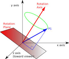
Compared to rotation matrices, quaternions are more compact, efficient, and numerically stable.
Compared to Euler angles, they are simpler to compose.
However, they are not as intuitive and easy to understand and, due to the periodic nature of sine and cosine, rotation angles differing precisely by the natural period will be encoded into identical quaternions and recovered angles in radians will be limited to [0, 2π]
We set our planeBody.quaternion.setFromEuler(-Math.PI / 2, 0, 0); in order to rotate the plane body to match the geometry, since our plane is rotated to be horizontal.
Lastly, we need to update the physics world in the animation loop.
We can do this by using delta time and the Cannon.js step function:
const clock = new THREE.Clock(); // Create a clock to track time
function animate() {
  requestAnimationFrame(animate);

  const deltaTime = clock.getDelta(); // Get the time elapsed since the last frame

  world.step(1 / 60, deltaTime, 3); // Step the physics world, parameters: time step, delta time, number of substeps

  // Update the Three.js objects to match the physics bodies
  sphereMesh.position.copy(sphereBody.position); // Update the sphere mesh position

  // Render the scene from the perspective of the camera
  renderer.render(scene, camera);

}

animate();
Now we have a simple physics simulation with a plane and a sphere.
The sphere will fall under the influence of gravity and collide with the plane.
We can increase the bounciness of the sphere by setting the restitution property, which is a measure of how much energy is conserved during a collision.
When two objects collide with each other, many forces come into play, which also means the application of various mathematical equations. Many of these laws were first derived by the same super popular scientist who is credited with numerous discoveries and derivations, meaning that he has a number of patents to his name -- Sir Isaac Newton.
Pertaining to the collision of two objects, Newton formulated a theory that we now know as Newton's law of restitution.
It simply states that when two bodies collide, the speed with which they move after the collision depends on the material from which they are made.
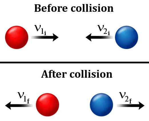
The coefficient of restitution (CoR) is a measure of how elastic a collision is between two objects.
It is defined as the ratio of the relative velocity of separation to the relative velocity of approach.
In simple terms, it tells us how much energy is conserved during a collision.
In most cases, the coefficient of restitution is between 0 and 1.

A coefficient of restitution of 1 means that the collision is perfectly elastic, meaning that no energy is lost during the collision. In other words, the objects will bounce off each other with the same speed and energy as they had before the collision.
A coefficient of restitution of 0 means that the collision is perfectly inelastic, meaning that all energy is lost during the collision and the objects stick together.
A coefficient of restitution between 0 and 1 means that the collision is partially elastic, meaning that some energy is lost during the collision.
Let's suppose a rubber ball bounces on a flat, hard surface. Obviously, the rubber ball will rebound off the surface, but with only a fraction of its original energy, because all real collisions are inelastic. (Note: If this collision were elastic, then the ball would have bounced back with the same amount of energy it had before striking the surface.)
When we 'deform' something by colliding it with something else (say, when we bounce a basketball on the ground), a fraction of its original energy is lost. That's why the basketball bounces lower with every collision -- as its energy gets converted to heat/vibrations.
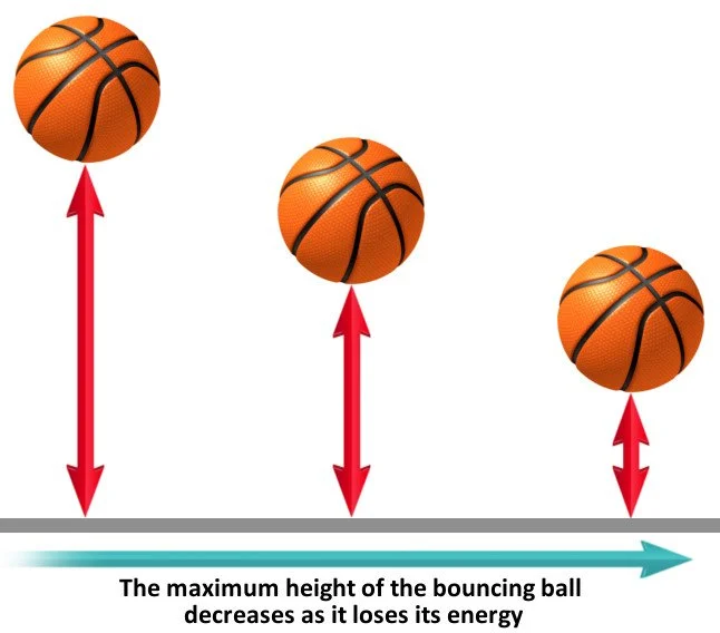
The formula to calculate the coefficient of restitution is rather straightforward. Since it is defined as a ratio of the final to the initial relative velocity between two objects after their collision, it can be mathematically represented as follows:

When considering a one-dimensional collision of two objects, A and B, the coefficient of restitution could be calculated by:
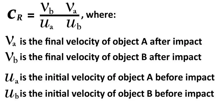
In the case of a ball bouncing off a flat, stationary surface, the coefficient of restitution turns out to be:

In the case of our sphere and plane, we can set the restitution property of the sphere to a value between 0 and 1 to control how bouncy the sphere is.
In Cannon.js, the restitution property is set on the material of the body.
We can create a new material for the plane and set the restitution property:
// Set restitution for the plane
planeBody.material = new CANNON.Material();
planeBody.material.restitution = 0.6; // Adjust this value for bounciness
And of the sphere:
// Set restitution for the sphere
sphereBody.material = new CANNON.Material();
sphereBody.material.restitution = 0.9; // Adjust this value for bounciness
Now the sphere will bounce off the plane when it collides.
Let's use what we know about raycasting to add the ability to pick up and drop the sphere.
We can do this by first creating a new raycaster to detect when the mouse is over the sphere and then pick it up.
// Raycaster and mouse
const raycaster = new THREE.Raycaster();
const mouse = new THREE.Vector2();
let isDragging = false; // Flag to check if the sphere is being dragged
We can write a function to handle the mouse down event:
function onMouseDown(event) {
  // Calculate mouse position in normalized device coordinates
  mouse.x = (event.clientX / window.innerWidth) * 2 - 1;
  mouse.y = -(event.clientY / window.innerHeight) * 2 + 1;

  // Update the picking ray with the camera and mouse position
  raycaster.setFromCamera(mouse, camera);

  // Calculate objects intersecting the picking ray
  const intersects = raycaster.intersectObject(sphereMesh);
  if (intersects.length > 0) {
    isDragging = true;
    sphereBody.velocity.set(0, 0, 0); // Reset velocity when picked up
  }
}
The onMouseDown function will be called when the mouse is clicked.
We can create another function to handle the mouse up event:
function onMouseUp() {
  if (isDragging) {
    isDragging = false;
    // Release the sphere and apply an initial force downward
    sphereBody.velocity.set(0, -2, 0); // Apply an initial downward velocity to simulate a bounce
  }
}
The onMouseUp function will be called when the mouse is released.
And finally, we can create a function to handle the mouse move event:
function onMouseMove(event) {
  if (isDragging) {
    // Calculate mouse position in normalized device coordinates
    mouse.x = (event.clientX / window.innerWidth) * 2 - 1;
    mouse.y = -(event.clientY / window.innerHeight) * 2 + 1;

    // Update the picking ray with the camera and mouse position
    raycaster.setFromCamera(mouse, camera);

    // Get the position in world coordinates
    const intersects = raycaster.intersectObject(planeMesh);
    if (intersects.length > 0) {
      const intersectPoint = intersects[0].point;
      // Set the sphere's position to be above the plane
      sphereBody.position.set(intersectPoint.x, intersectPoint.y + 2, intersectPoint.z); // Keep it above the plane
      sphereMesh.position.copy(sphereBody.position); // Sync visual sphere position
    }
  }
}
Which will be called when the mouse is moved.
We can add event listeners to the document to handle the mouse events:
document.addEventListener("mousedown", onMouseDown, false);
document.addEventListener("mouseup", onMouseUp, false);
document.addEventListener("mousemove", onMouseMove, false);
Now we can pick up and drop the sphere using the mouse.
We can add more objects to the scene and create more complex physics simulations.
We can also create more complex objects and add them to the scene.
Let's start by setting up our Physics world:
// Initialize physics world
const world = new CANNON.World();
world.gravity.set(0, -9.81, 0);
We can also create our clock for delta time and step our physics world in our animate function:
// Animation loop
const clock = new THREE.Clock();

function animate() {
  requestAnimationFrame(animate);
  const delta = clock.getDelta();

  // Step the physics world
  world.step(1 / 60, delta, 3);

  renderer.render(scene, camera);
}

animate();
Now we can create our plane (in both the scene and our Physics World). However, by default, CANNON.Plane() is an infinite plane, but its orientation and the shape's effective size are not directly set by dimensions like in THREE.PlaneGeometry. To get a finite plane matching our visual plane size, we will use CANNON.Box:
// Define size for the visual and physics ground plane
const planeSize = 25;

// --- Visual Ground Plane ---
const planeGeo = new THREE.PlaneGeometry(planeSize, planeSize);
const planeMat = new THREE.MeshStandardMaterial({
  color: "lightgrey",
  side: THREE.DoubleSide
});
const planeMesh = new THREE.Mesh(planeGeo, planeMat);
planeMesh.rotation.x = -Math.PI / 2;
planeMesh.receiveShadow = true;
scene.add(planeMesh);

// --- Physics Ground Plane ---
// Using a box shape to match the visual plane's size
const groundShape = new CANNON.Box(
  new CANNON.Vec3(planeSize / 2, 0.1, planeSize / 2)
);
const groundBody = new CANNON.Body({ mass: 0 });
groundBody.addShape(groundShape);
groundBody.position.set(0, 0, 0);
world.addBody(groundBody);
Now we can start adding in our objects:
// Arrays to hold visual meshes and physics bodies
const objects = [];
const physicsBodies = [];

// Create a wall of cubes
const rows = 7;
const cols = 15;
const cubeSize = 1;
const startX = -(cols / 2) * cubeSize + cubeSize / 2;
const startY = -0.5;
const startZ = 0;

for (let i = 0; i < rows; i++) {
  for (let j = 0; j < cols; j++) {
    const x = startX + j * cubeSize;
    const y = startY + i * cubeSize;
    const z = startZ;

    // Visual cube
    const geo = new THREE.BoxGeometry(cubeSize, cubeSize, cubeSize);
    const mat = new THREE.MeshStandardMaterial({ color: 0x00ff00 });
    const mesh = new THREE.Mesh(geo, mat);
    mesh.castShadow = true;
    scene.add(mesh);
    objects.push(mesh);

    // Physics body
    const shape = new CANNON.Box(
      new CANNON.Vec3(cubeSize / 2, cubeSize / 2, cubeSize / 2)
    );
    const body = new CANNON.Body({ mass: 0.5 });
    body.addShape(shape);
    body.position.set(x, y, z);
    world.addBody(body);
    physicsBodies.push(body);
  }
}
We will see a wall of cubes with 7 rows and 15 cubes per row once we update our animate function:
for (let i = 0; i < physicsBodies.length; i++) {
    const pBody = physicsBodies[i];
    const mesh = objects[i];
    mesh.position.copy(pBody.position);
    mesh.quaternion.copy(pBody.quaternion);
}
We want to be able to shoot balls at the wall to knock down the cube, this will require a raycaster:
// For shooting balls
const ballRadius = 0.5;
const ballGeometry = new THREE.SphereGeometry(ballRadius, 16, 16);
const ballMaterial = new THREE.MeshStandardMaterial({ color: 0xff0000 });

const ballMeshes = [];
const ballBodies = [];

// Raycaster for mouse interaction
const raycaster = new THREE.Raycaster();
const mouse = new THREE.Vector2();

function onMouseDown(event) {
  // Convert mouse coords
  mouse.x = (event.clientX / window.innerWidth) * 2 - 1;
  mouse.y = -(event.clientY / window.innerHeight) * 2 + 1;

  // Raycast from camera
  raycaster.setFromCamera(mouse, camera);
  const direction = raycaster.ray.direction.clone();
  const origin = raycaster.ray.origin.clone();

  // Create visual sphere
  const mesh = new THREE.Mesh(ballGeometry, ballMaterial);
  mesh.castShadow = true;
  scene.add(mesh);
  ballMeshes.push(mesh);

  // Create physics body
  const shape = new CANNON.Sphere(ballRadius);
  const body = new CANNON.Body({ mass: 1 });
  body.addShape(shape);

  // Position the ball slightly in front of camera
  const spawnPos = origin.clone().add(direction.clone().multiplyScalar(1));
  body.position.copy(spawnPos);
  // Set initial velocity forward
  const shootSpeed = 50;
  body.velocity.copy(direction.multiplyScalar(shootSpeed));

  world.addBody(body);
  ballBodies.push(body);
}

document.addEventListener("mousedown", onMouseDown);
Now we should possess the ability to shoot balls at our scene. Let's modify our animate function to reflect this:
for (let i = 0; i < ballBodies.length; i++) {
    ballMeshes[i].position.copy(ballBodies[i].position);
    ballMeshes[i].quaternion.copy(ballBodies[i].quaternion);
}
And now we should be able to knock down the cubes with the spheres!
We can also use Cannon.js to create more advanced physics simulations, such as ragdoll physics, soft body physics, and fluid dynamics.
So we spoke about the two main cameras in Three.js, the PerspectiveCamera and the OrthographicCamera, but what exactly are they?
The PerspectiveCamera, as we know, is the most commonly used camera in Three.js. It mimics the perspective projection of real-world cameras, creating a sense of depth and realism in the scene. So that the objects far from the camera look smaller and those near to the camera look bigger, just like our eyes work.
Once again, it is defined by a field of view (FOV), aspect ratio, and near and far clipping planes.
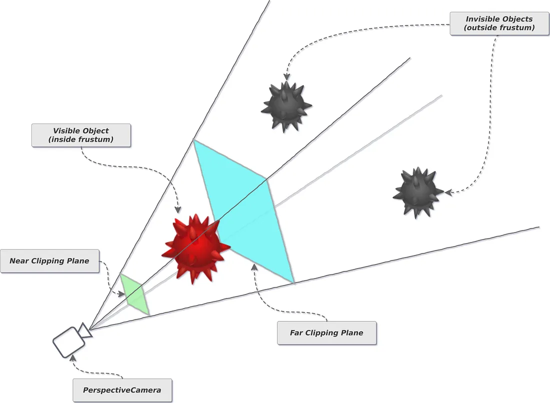
Let's set up a scene that uses a PerspectiveCamera:
const scene = new THREE.Scene();
scene.background = new THREE.Color("green");

// Set up the Camera (Perspective)
const camera = new THREE.PerspectiveCamera(
  75, // Field of view (in degrees)
  window.innerWidth / window.innerHeight, // Aspect ratio
  0.1, // Near clipping plane
  1000 // Far clipping plane
);

// Position the camera
camera.position.set(3, 5, 7);
camera.lookAt(0, 0, 0);

const renderer = new THREE.WebGLRenderer({ antialias: true }); // Add antialiasing
renderer.setSize(window.innerWidth, window.innerHeight);
renderer.shadowMap.enabled = true; // Enable shadow maps
renderer.shadowMap.type = THREE.PCFSoftShadowMap; // Softer shadows
document.body.appendChild(renderer.domElement);

// Create the Plane
const planeGeometry = new THREE.PlaneGeometry(20, 20); // Larger plane
const planeMaterial = new THREE.MeshStandardMaterial({
  color: "lightgrey",
  side: THREE.DoubleSide
});
const plane = new THREE.Mesh(planeGeometry, planeMaterial);
plane.rotation.x = Math.PI / 2; // Rotate to lie flat
plane.receiveShadow = true; // Plane can receive shadows
scene.add(plane);

// Create the Cube
const cubeGeometry = new THREE.BoxGeometry(1, 1, 1); // Width, height, depth
const cubeMaterial = new THREE.MeshStandardMaterial({ color: "blue" });
const cube = new THREE.Mesh(cubeGeometry, cubeMaterial);
cube.position.set(-1.5, 0.5, 0); // Position above the plane
cube.castShadow = true; // Cube can cast shadows
scene.add(cube);

// Create the Sphere
const sphereGeometry = new THREE.SphereGeometry(0.75, 32, 16); // Radius, width segments, height segments
const sphereMaterial = new THREE.MeshStandardMaterial({ color: 0xff0000 }); // Red color
const sphere = new THREE.Mesh(sphereGeometry, sphereMaterial);
sphere.position.set(1.5, 0.75, 0); // Position above the plane
sphere.castShadow = true; // Sphere can cast shadows
scene.add(sphere);

// Add Lighting
const ambientLight = new THREE.AmbientLight("grey", 0.5); // Color, Intensity
scene.add(ambientLight);

const directionalLight = new THREE.DirectionalLight("white", 0.8); // Color, Intensity
directionalLight.position.set(5, 10, -10); // Position of the light source
directionalLight.castShadow = true; // Enable shadow casting for this light

scene.add(directionalLight);

function animate() {
  requestAnimationFrame(animate);
  renderer.render(scene, camera);
}

animate();
The OrthographicCamera, on the other hand, provides an orthographic projection, which means that objects appear the same size regardless of their distance from the camera. This camera type is often used for 2D games or architectural visualizations.
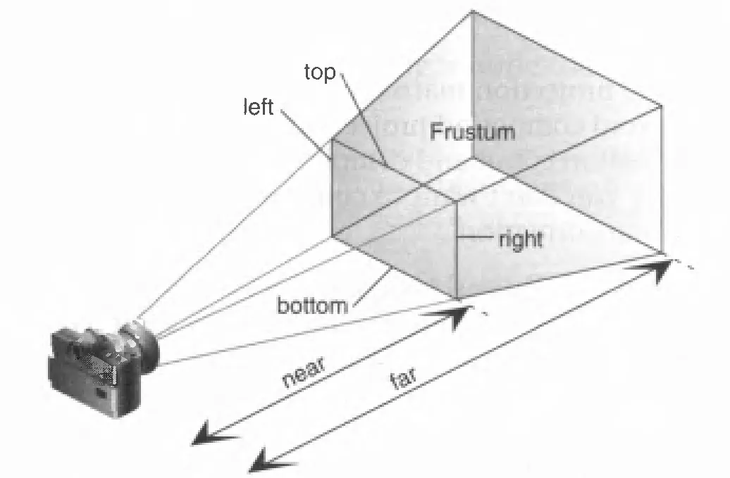
To create an OrthographicCamera in Three.js, we can use the following constructor:
const camera = new THREE.OrthographicCamera(left, right, top, bottom, near, far);Where:
We can modify our cube and sphere scene to use an OrthographicCamera instead:
//Set up the Camera (Orthographic)
const aspect = window.innerWidth / window.innerHeight;
const frustumSize = 15; // Controls the 'zoom' or size of the view
const camera = new THREE.OrthographicCamera(
  (frustumSize * aspect) / -2, // left
  (frustumSize * aspect) / 2, // right
  frustumSize / 2, // top
  frustumSize / -2, // bottom
  -100, // Near clipping plane
  1000 // Far clipping plane
);
Orthographic projection is just one of the types of parallel projection.
Representing an n-dimensional object into an n-1 dimension is known as projection.
It is process of converting a 3D object into 2D object, where we represent a 3D object on a 2D plane {(x,y,z)->(x,y)}. It is also defined as mapping or transforming of the object in projection plane or view plane.
When geometric objects are formed by the intersection of lines with a plane, the plane is called the projection plane and the lines are called projections.

The center of projection (CoP) is an arbitrary point from where the lines are drawn on each point of an object.
A parallel projection is formed by extending parallel lines from each vertex of object until they intersect plane of screen.
Parallel projection transforms object to the view plane along parallel lines. A projection is said to be parallel, if center of projection is at an infinite distance from the projected plane.
A parallel projection preserves relative proportion of objects, accurate views of the various sides of an object are obtained with a parallel projection. The projection lines are parallel to each other and extended from the object and intersect the view plane.
It preserves relative propositions of objects, and it is used in drafting to produce scale drawings of 3D objects. This is not a realistic representation, the point of intersection is the projection of the vertex.
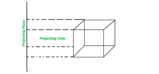
Parallel projection is divided into two parts and these two parts sub divided into many:
In orthographic projection the direction of projection is normal to the projection of the plane. In orthographic lines are parallel to each other making an angle 90 with view plane. Orthographic parallel projections are done by projecting points along parallel lines that are perpendicular to the projection line.
Orthographic projections are most often used to procedure the front, side, and top views of an object and are called evaluations.
Engineering and architectural drawings commonly employ these orthographic projections.
Transformation equations for an orthographic parallel projection as straight forward. Some special orthographic parallel projections involve plan view, side elevations. We can also perform orthographic projections that display more than one phase of an object, such views are called monometric orthographic projections.
Multiview Projection is further divided into three categories:
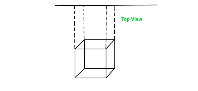
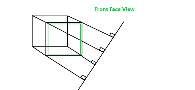
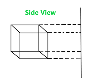
Axonometric projection is an orthographic projection, where the projection lines are perpendicular to the plane of projection, and the object is rotated around one or more of its axes to show multiple sides.
It is further divided into three categories:
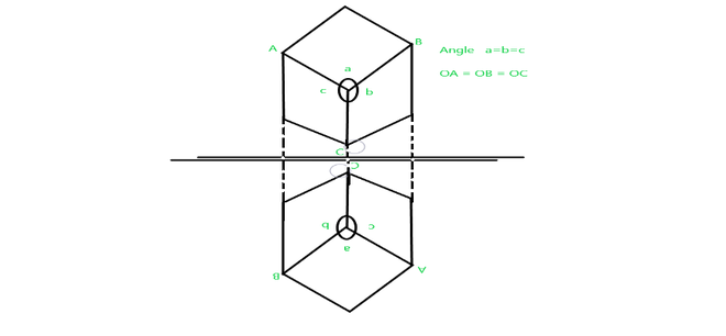

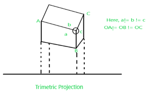
Oblique projection is a kind of parallel projection where projecting rays emerges parallel from the surface of the polygon and incident at an angle other than 90 degrees on the plane.
It is further divided into two categories:
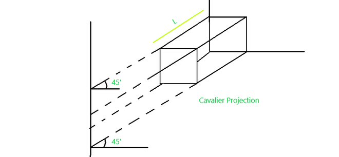
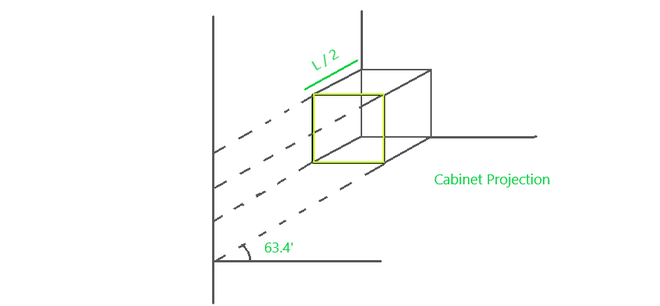
In Perspective Projection the center of projection (CoP) is at finite distance from projection plane.
The perspective projection can be easily described by the following figure:
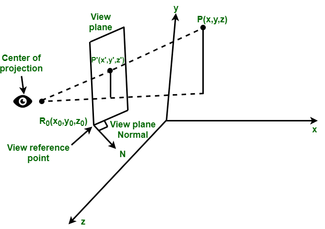
This projection produces realistic views but does not preserve relative proportions of an object dimensions. Projections of distant object are smaller than projections of objects of same size that are closer to projection plane.
In perspective projection, the lines of projection are not parallel. Instead, they all converge at a single point called the center of projection or projection reference point.
The object positions are transformed to the view plane along these converged projection lines and the projected view of an object is determined by calculating the intersection of the converged projection lines with the view plane, as shown in the below figure:
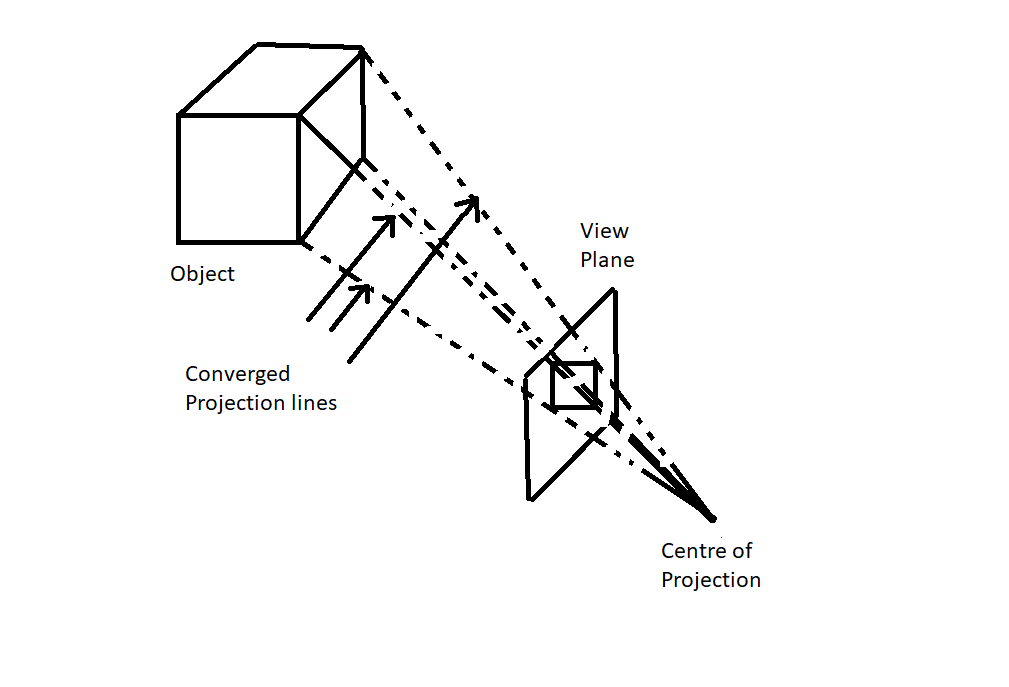
Classification of perspective projection is on basis of vanishing points (It is a point in image where a parallel line through center of projection intersects view plane.).
The classification is as follows:

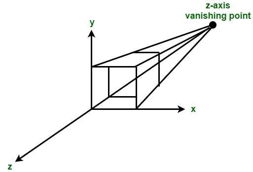

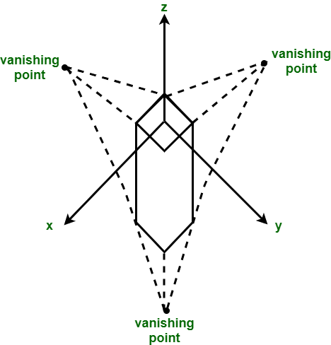
There are also other types of cameras in Three.js, such as the CubeCamera, which is used for rendering cube maps, and the StereoCamera, which is used for rendering stereo images for VR applications.
As we have already seen, the CubeCamera is used for capturing a panoramic view of the scene from a specific position. It renders the scene six times, each time capturing the view along one of the cube's faces. This camera type is commonly used for creating reflections or environment maps.
Here’s an example of creating and updating a CubeCamera:
const cubeCamera = new THREE.CubeCamera(near, far, resolution);Where:
To use the CubeCamera, you need to add it to the scene and update it in your render loop:
// Add the CubeCamera to the scene
scene.add(cubeCamera);

// Update the CubeCamera in the render loop
cubeCamera.update(renderer, scene);
CubeCamera is useful for creating realistic reflections and environment maps in your 3D scenes.
The ArrayCamera allows you to create an array of cameras and switch between them to achieve different perspectives or views. It can be useful for creating multi-camera setups or implementing camera transitions.
To create an ArrayCamera, you can use the following constructor:
const cameras = [
  new THREE.PerspectiveCamera(fov, aspect, near, far),
  new THREE.PerspectiveCamera(fov, aspect, near, far)
];
const arrayCamera = new THREE.ArrayCamera(cameras);
Where:
To use the ArrayCamera, you can set it as the active camera in your render loop:
// Set the ArrayCamera as the active camera
renderer.render(scene, arrayCamera);
ArrayCamera is useful for creating multi-camera setups or implementing camera transitions in your 3D scenes.
The StereoCamera is used to create stereoscopic 3D effects, providing a sense of depth perception by rendering separate views for the left and right eye. This camera type is commonly used for virtual reality (VR) or augmented reality (AR) applications.
It is used to render the scene through two cameras that mimic the eyes in order to create what we call a parallax effect that will lure your brain into thinking that there is depth. You must have the adequate equipment like a VR headset or red and blue glasses to see the result.
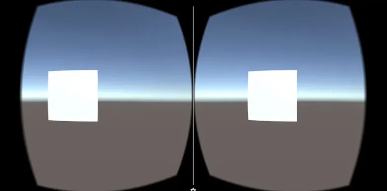
Here’s an example of creating a StereoCamera:
const camera = new THREE.StereoCamera();

// Set up left and right cameras
const leftCamera = camera.cameraL;
const rightCamera = camera.cameraR;

// Position the cameras
leftCamera.position.set(x, y, z);
rightCamera.position.set(x, y, z);

// Set the focal length for both cameras
leftCamera.focalLength = 10;
rightCamera.focalLength = 10;
To render the stereo view, you need to update the camera and render the scene twice, once for the left eye and once for the right eye.
Here’s an example of rendering with a StereoCamera, we would put the following in our animate() function:
// Update the stereo camera
camera.update(renderer, scene);

// Set the active renderer to the left eye
renderer.setRenderTarget(renderer.getRenderTarget().left);
renderer.render(scene, leftCamera);

// Set the active renderer to the right eye
renderer.setRenderTarget(renderer.getRenderTarget().right);
renderer.render(scene, rightCamera);

// Reset the active renderer to the default
renderer.setRenderTarget(null);
Understanding the different types of cameras available in Three.js is crucial for controlling the view and perspective of our 3D scenes.
Whether we need to create a realistic perspective, an orthographic projection, or capture panoramic views, Three.js offers a variety of camera options to suit our needs. By utilising these cameras, we can enhance the interactivity and immersion of our web-based 3D applications.
Remember to experiment with camera settings, position, and movement to achieve the desired effects and create captivating user experiences.
So we have created objects and added textures to them, but how do we create our own custom shaders?
Shaders are small programs that run on the GPU (Graphics Processing Unit) and are used to control the rendering process in Three.js. They allow us to create custom visual effects, manipulate vertex positions, and control how materials are rendered.
These programs are run for each specific section of the graphics pipeline. In a basic sense, shaders are nothing more than programs transforming inputs to outputs. Shaders are also very isolated programs in that they're not allowed to communicate with each other; the only communication they have is via their inputs and outputs.
Shaders are written in the language GLSL.
GLSL stands for OpenGL Shading Language, a high-level shading language used for programming graphics shaders within the OpenGL API. It's a C-style language that allows developers to control the rendering pipeline on the GPU, enabling the creation of complex visual effects and graphics. GLSL shaders are executed on the GPU and are crucial for rendering 2D and 3D graphics in applications and games
GLSL is tailored for use with graphics and contains useful features specifically targeted at vector and matrix manipulation.
Shaders always begin with a version declaration, followed by a list of input and output variables, uniforms and its main function. Each shader's entry point is at its main function where we process any input variables and output the results in its output variables. Don't worry if you don't know what uniforms are, we'll get to those shortly.
Same as the other programming languages, GLSL utilizes variables for storing information.
However, it's essential to declare the data type of the variable before use, unlike JavaScript, where types are inferred. This explicit declaration ensures strict type handling.
int a = 77;In addition to variables, we have constants, which are variables that must be initialized upon declaration and cannot be updated afterward.
The main difference between constants in GLSL and JavaScript lies in the requirement to specify the data type in GLSL. Otherwise, their behavior is similar.
const int b = 50.0;GLSL supports a variety of data types, including:
Unlike some other languages, GLSL does not include character or string types.
int a = 77;
const float b = 50.0;
bool c = true;
Once a variable is assigned a data type, it cannot be reassigned a value of a different type. For instance, it's not possible to assign a float value to an int variable or vice versa, ensuring strict adherence to data types.
// These couple lines generate error messages.
int a = 20.0;
float b = 4;
The only way to assign the value of a variable to another one with a different type is by using a type conversion function.
For instance, you can convert a float value to an integer using the int() function.
float x = 4.0;
int y = 20;
bool z = false;

// a = 4
int a = int(x);
// b = 20.0
float b = float(y);
// c = 0.0
float c = float(z);
In addition to variables and type conversions, we have a variety of operators for performing different operations such as addition (+), subtraction (-), division (/), and more.
// a = 4
int a = 2 + 2;
// a = 5
a++;GLSL also supports vectors and matrices, which are essential for representing points, colors, and other attributes in 3D space. hese types are analogous to objects in object-oriented languages, as they are composed of basic types and allow for more complex operations.
Vectors are categorized into three types:
Each type is designed to handle specific kinds of data.
In addition to specifying the type, we need to use a digit to indicate the number of components in a vector.
A vector can have a minimum of 2 components and a maximum of 4 components.
vec2 vectA = vec2(1.0, 5.0);
ivec3 vectB = ivec3(7, 10, 1);
bvec4 vectC = bvec4(true, true, false, false);
In the above example, we have a 2D vector (vec2), a 3D vector (ivec3), and a 4D vector (bvec4).
Another way to create a vector, when all its components have the same value, is by specifying that value only once.
// Same as: vec3 vectD = vec3(0.0, 0.0, 0.0);
vec3 vectD = vec3(0.0);
We can also initialize a vector by using the values from another vector.
vec2 vectE = vec2(3.0, 9.0);
// Same as: vec4 vectF = vec4(3.0, 9.0, 0.0, 10.0);
vec4 vectF = vec4(vectE, 0.0, 10.0);
// Same as: vec2 vectG = vec3(3.0, 9.0);
vec2 vectG = vec2(vectF);
Furthermore, we can combine values from multiple vectors to create a new vector.
bvec2 vectH = bvec2(true);
bvec2 vectI = bvec2(false);
// Same as: bvec4 vectJ = bvec4(true, true, false, false);
bvec4 vectJ = bvec4(vectH, vectI);
To access the first component of a vector, specify the variable name followed by a period and then x, r, or s.
vec4 v = vec4(2.0, 3.0, 7.0, 5.0);
// a == b == c == 2.0
float a = v.x;
float b = v.r;
float c = v.s;
To access the second component of a vector, use the variable name followed by a period and then y, g, or t.
vec4 v = vec4(2.0, 3.0, 7.0, 5.0);
// a == b == c == 3.0
float a = v.y;
float b = v.g;
float c = v.t;To access the third component of a vector, use the variable name followed by a period and then z, b, or p.
vec4 v = vec4(2.0, 3.0, 7.0, 5.0);
// a == b == c == 7.0
float a = v.z;
float b = v.b;
float c = v.p;To access the fourth component of a vector, use the variable name followed by a period and then w, a, or q.
vec4 v = vec4(2.0, 3.0, 7.0, 5.0);
// a == b == c == 5.0
float a = v.w;
float b = v.a;
float c = v.q;As you can see, there are various notations for accessing vector components, each suited for different contexts.
For example:
It's important to note that we can access multiple components of a vector simultaneously. For example, we can create a new vector whose components are taken from the 1st and 3rd components of another vector.
vec4 vectA = vec4(2.0, 3.0, 7.0, 5.0);
// Same as: vec2 vectB = vec2(2.0, 7.0);
vec2 vectB = vectA.xz;Also we have the flexibility to repeat values or rearrange them in a different order within vectors.
vec4 vectA = vec4(2.0, 3.0, 7.0, 5.0);
// Same as: vec3 vectB = vec3(2.0, 2.0, 2.0);
vec3 vectB = vectA.rrr;
// Same as: vec2 vectC = vec2(7.0, 2.0);
vec3 vectC = vectA.br;Quite similar to vectors, a matrix is composed of a certain number of floats. So we have mat2, mat3, and mat4 matrices.
Unlike vectors, matrices can contain different types of values simultaneously. For example, a mat2 could theoretically have 2 integers and 2 booleans. However, these values will be converted automatically into floats.
// Same as: mat2 mat = mat2(1.0, 1.0, 0.0, 0.0);
mat2 mat = mat2(1, 1, false, false);The elements of a matrix are set in a column-major order. This means that when creating a matrix with code, the elements must be typed in column order.
To access the components of a matrix, we use bracket notation. For example, m[0] accesses the first column of a matrix m and returns it as a vector.
mat3 m = mat3(7.0, 4.0, 5.0, 0.0, 2.0, 0.5, 1.0, 3.0, 7.0);
// Same as: vec3 v = vec3(7.0, 4.0, 5.0);
vec3 v = m[0];To set the last value of a matrix m to 100, you can use double brackets m[2][2].
mat3 m = mat3(7.0, 4.0, 5.0, 0.0, 2.0, 0.5, 1.0, 3.0, 7.0);
m[2][2] = 100.0;Furthermore, we can combine the dot notation used to get and set vector values with bracket notation for matrices.
mat3 m = mat3(7.0, 4.0, 5.0, 0.0, 2.0, 0.5, 1.0, 3.0, 7.0);
// f value is 4.0
// Same as: float f = m[0][1];
float f = m[0].y;Of course, we can perform a variety of operations on vectors and matrices just as we do with other types. This includes addition, subtraction, multiplication, and more. For instance, you can add two vectors, multiply a matrix by a vector, or even multiply two matrices together.
Another type of variables we have is sampler. Actually we have a couple of them: sampler2D, which you will use most often for 2D textures, and samplerCube, which is used for cube map textures.
In short, a sampler is a type of variable used to store image data in GLSL.
Similar to other programming languages, GLSL provides arrays to store collections of data.
To create an array, we need to specify the type and the number of elements in advance.
In the example below, the number 7 does not initialize the array with the value 7; instead, it indicates that the array can hold up to 7 elements.
float arr[7];To access an element of an array, we use bracket notation in the same way as in C or JavaScript.
float arr[7];
// Sets the value of the first element
arr[0] = 20.0;
// Gets the value of the last element
float f = arr[6];In addition to the different types of variables we've seen, GLSL also allows us to create our own custom types.
To create custom types, we use the keyword struct, followed by a name and a pair of opening and closing curly braces. Within these braces, we specify the components of our structure, defining our custom type.
struct myType {
int c1;
vec3 c2;
};Once we've defined the structure of our custom type, creating a variable of that type is done in the same way as with other variable types.
struct myType {
int c1;
vec3 c2;
};
myType a;To access the components of a variable of a custom type, whether to get or set their values, we use the dot notation, similar to how we access components of vectors.
struct myType {
int c1;
vec3 c2;
};
myType a;
// Sets the value of c1
a.c1 = 10;
// Gets the value of c2
vec3 v = a.c2;Again similar to other programming languages, we have control flow statements such as if-else statements, switch cases, for loops, and while loops.
if(condition1) {
// Do something
} else if(condition2) {
// Do something else
} else {
// Do something else
}for(int i = 0; i < 10; i++) {
// Do something
}A function in GLSL, like a variable, must have a type. If a function returns a value, its type must match the type of the returned value. However, if a function doesn't return anything, its type must be set to void.
void funcA() {
// Stuff to do
}
float funcB() {
// Stuff to do
return 1.0;
}It is also necessary to specify the types of parameters for a function.
float func(vec3 v) {
return v.x;
}It's crucial to note that function definitions must be placed outside the main function. More on the main function later on.
float func(vec3 v) {
return v.x;
}
void main() {
// Stuff to do
}In GLSL, the order of function definition and calling matters. Functions need to be defined before they are called.
// This works
int func() {
return 5;
}
void main() {
int five = func();
}// This won't work!
void main() {
int five = func();
}
int func() {
return 5;
}That said, we can actually do something to bypass this rule.
To do that, we can set what is called the prototype of the function at the top of the code. A prototype is essentially the definition of the function without its body. We can then call the function and provide its full definition at the bottom of the code base.
// This is the prototype of the function
vec2 func(float x, float y);
void main() {
vec2 v = func(2.0, 3.0);
}
vec2 func(float x, float y) {
return vec2(x, y);
}GLSL provides a wealth of built-in functions. For comprehensive documentation on these functions, be sure to visit shaderific.com. There, you'll find brief documentation for any built-in function you might need.
There are four storage qualifiers. We have already encountered one of them: const. The other three are attribute, uniform, and varying.
Attribute and uniform variables, are variables that receive data from the outside of the GLSL code, from the Javascript side of the application code more precisely.
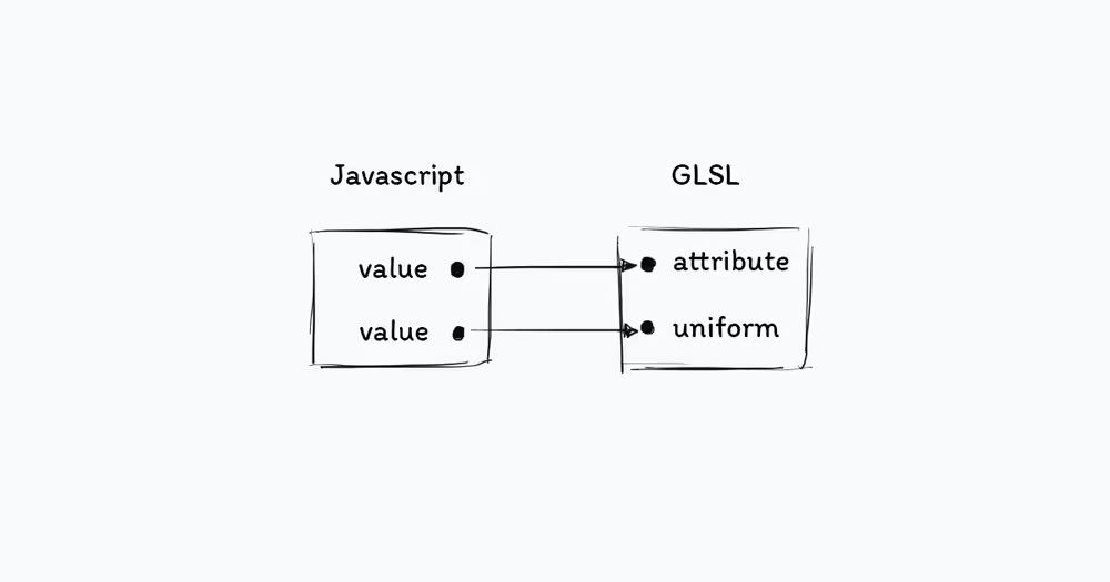
The difference between the two is that an attribute variable holds data that varies from one vertex to another.
In contrast, time should be passed as a uniform variable because all vertices share the same time value.
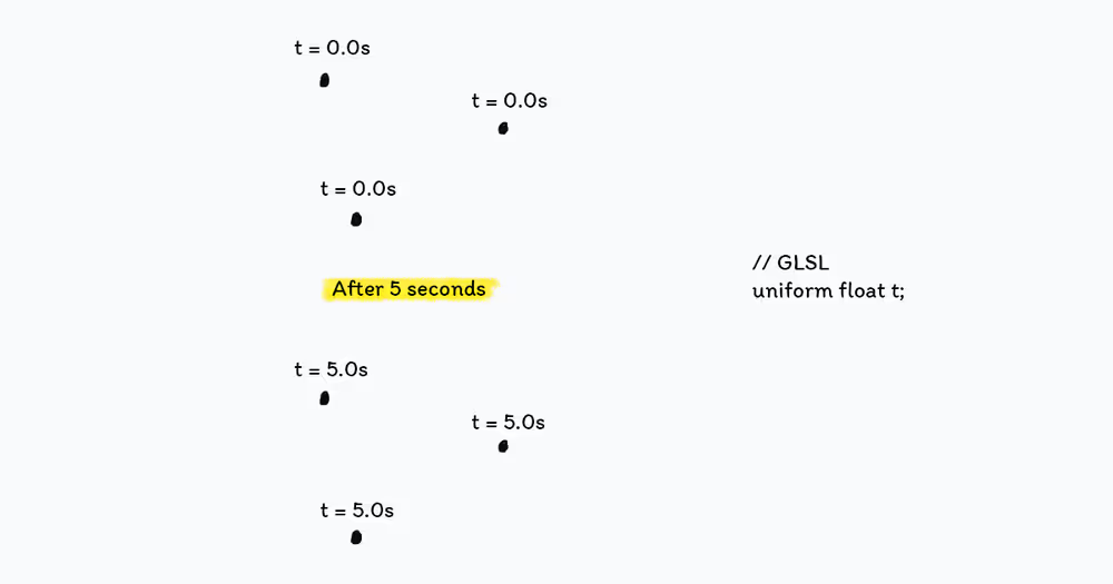
Another difference between attributes and uniforms is that the number of attribute variables allowed is less than the number of uniforms.
Additionally, attribute variables can only be used in the vertex shader, while uniforms are allowed in both the vertex and fragment shaders.
Varying variables, on the other hand, are used to transfer data from the vertex shader to the fragment shader. That's it.
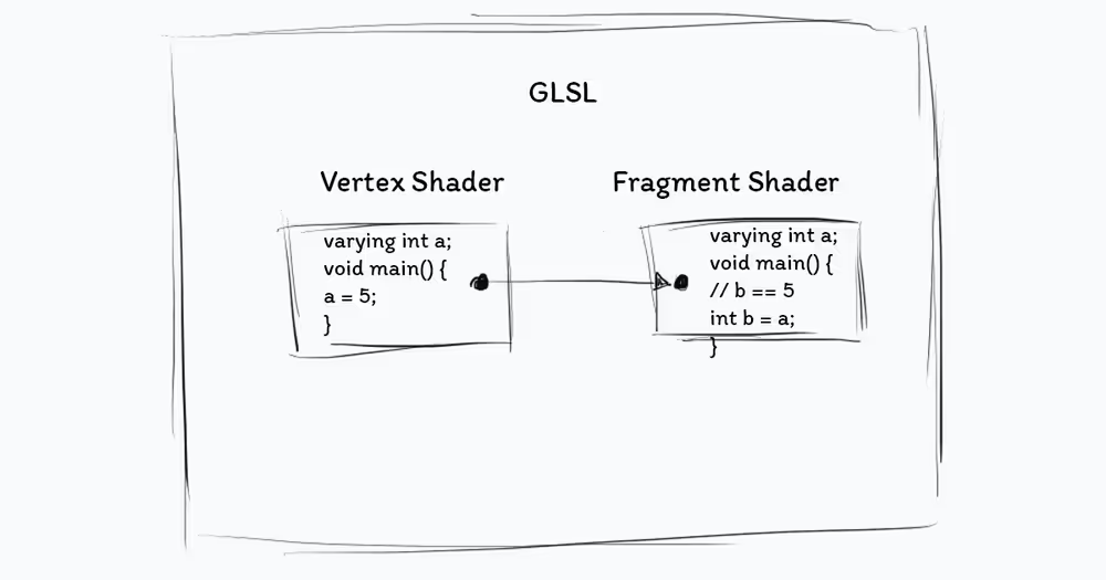
Precision qualifiers are used to optimize resource consumption, specifically memory usage.
There are three precision qualifiers: lowp, mediump, and highp, with lowp being the least resource-intensive. However, it's important to carefully choose the right precision, as a lower precision can sometimes yield incorrect results.
To set the precision of a variable, simply begin its declaration with the desired precision qualifier.
mediump float f = 5.0;Alternatively, you can set a precision for an entire type of variables by using the keyword precision, followed by the precision qualifier, and then the type.
precision highp int;WebGL does not offer the use of the Fixed Pipeline, which is a shorthand way of saying that it doesn't give you any means of rendering your stuff out of the box.
What it does offer, however, is the Programmable Pipeline, which is more powerful but which can also be more challenging to understand and use.
In the programmable pipeline, you have to write your own shaders to do the rendering. This is where the vertex and fragment shaders come into play.
What you should know about them is that they both run entirely on your graphics card's GPU. This means that we want to offload all that we can to them, leaving our CPU to do other work. A modern GPU is heavily optimised for the functions that shaders require so it's great to be able to use it.
Take a standard primitive shape, like a sphere. It's made up of vertices, right?
Every object in 3D, whether it's a point, text, shape, or a 3D model, is composed of a number of vertices. The role of a vertex shader is to handle the positioning of each vertex comprising that mesh in the scene.
In and of itself that's quite an interesting process, because we're actually talking about getting a 3D position (a vertex with x,y,z) onto, or projected, to a 2D screen. Thankfully for us if we're using something like Three.js we will have a shorthand way of setting the gl_Position without things getting too tricky.
The code of a vertex shader must be enclosed within a function named main. This function will be executed once for each vertex that composes the mesh.
void main() {
// Vertex shader logic
}For example, if we create an object with 20 vertices, the main function of the vertex shader will be executed 20 times to position each vertex correctly.
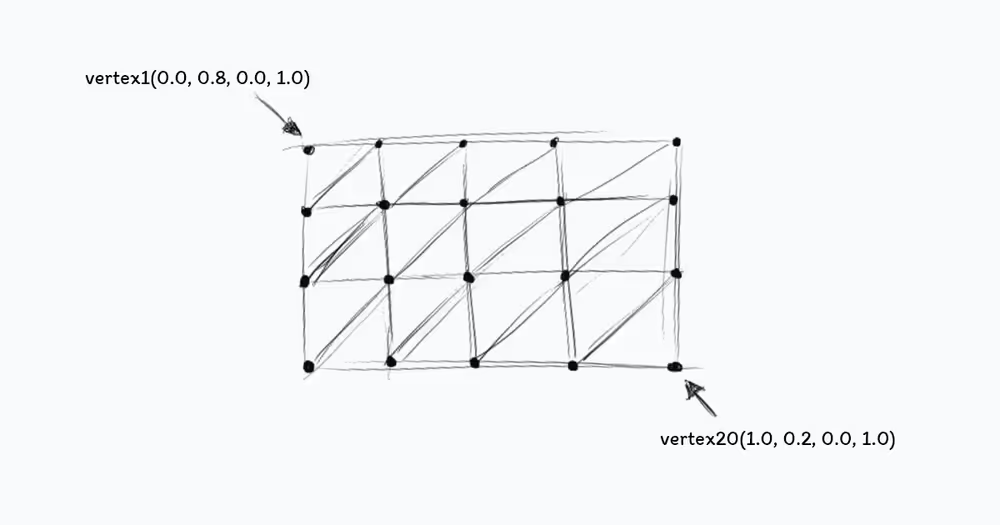
Within the main function of the vertex shader, we must assign a value to the built-in variable gl_Position, which indicates the coordinates of each vertex.
void main() {
// Stuff to do
gl_Position = projectionMatrix * modelViewMatrix * vec4(position, 1.0);
}The value of gl_Position here depends on the 3D library you're using.
In Three.js the gl_Position value depends on projectionMatrix, modelViewMatrix, and position which are Three.js built-in variables.
The first two variables, projectionMatrix and modelViewMatrix, are related to the camera view and contribute to the calculation of the final value passed to gl_Position.
The third variable, position, stores the initial coordinates of a vertex. It's important to note that this may vary if you're working with a different library, such as Babylon.js or Pixi.js.
Essentially, the role of a fragment shader is to apply colors to vertices and the meshes they form after they have been positioned by the vertex shader.
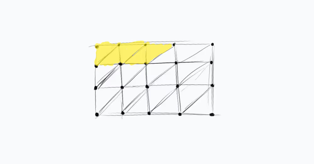
The colorization process involves several steps, but as a beginner, you just need to know that the fragment shader breaks down the mesh, created from the vertices positioned by the vertex shader, into small fragments and then colorizes them.
Similar to the vertex shader, a fragment shader's code must be enclosed within the body of a main function. Within this function, we also need to specify a special built-in variable called gl_FragColor.
void main() {
// Stuff to do
gl_FragColor = vec4(1.0, 1.0, 1.0, 1.0);
}As its name suggests, gl_FragColor is where the color of one fragment is stored. This vec4 variable has four components, each representing a color channel: the first value represents the red channel, the second the green channel, the third the blue channel, and the fourth the alpha channel.
Bear in mind that the values of these components range from 0 to 1. Any negative value is treated as 0, and any value exceeding 1 is equivalent to 1.
First, we need a basic Three.js project to implement what we've learned so far. To make things easier, here's a basic Three.js scene.
Every object in a Three.js scene has its own vertex and fragment shader. In fact, even the scene itself has a vertex and fragment shader. To apply an effect using shaders, we will replace the existing shaders with the custom ones we write.
Shaders are passed to meshes as custom materials. So to apply a specific effect to a mesh, you need to create a new material with a vertex and fragment shader, then combine this material with the geometry to create the mesh.
To create the custom material, We'll instantiate a new instance of the ShaderMaterial class.
The ShaderMaterial constructor takes an object as an argument, where we specify the code for our vertex and fragment shaders, along with other configurations such as wireframe mode.
Let's create a plane to do this:
const planeGeometry = new THREE.PlaneGeometry(10, 10, 30, 30);
const planeCustomMaterial = new THREE.ShaderMaterial({
vertexShader: `// Vertex shader code here`,
fragmentShader: `// Fragment shader code here`,
wireframe: true
});
const planeMesh = new THREE.Mesh(
planeGeometry,
planeCustomMaterial
);
scene.add(planeMesh);A good practice is to separate your GLSL logic from your JavaScript code for clarity and organization. You can create separate files for the vertex and fragment shaders, or you can place them in the HTML as script tags. We'll use the script tag option.
Let's add our vertex and fragment shaders in our HTML:
<script id="vertexshader" type="vertex">
void main() {
gl_Position = projectionMatrix * modelViewMatrix * vec4(position, 1.0);
}
</script>
<script id="fragmentshader" type="fragment">
void main() {
gl_FragColor = vec4(1.0);
}
</script>Now we'll pass the values of these script tags to the vertex and fragment shaders properties using their ids.
const planeCustomMaterial = new THREE.ShaderMaterial({
vertexShader: document.getElementById('vertexshader').textContent,
fragmentShader: document.getElementById('fragmentshader').textContent,
side: THREE.DoubleSide,
wireframe: true
});Now we should see a white wireframe plane in the scene. The vertex shader is responsible for positioning the vertices of the plane, while the fragment shader colors them.
Let's use the vertex shader to reposition the vertices that form our plane.
To do this, we simply need to update the value of the position variable, which is of type vec since it contains the x, y, and z positions of a vertex. We'll apply the sin() math function here.
<script id="vertexshader" type="vertex">
void main() {
// sin() is applied to the x, y, z components of the position vector
gl_Position = projectionMatrix * modelViewMatrix * vec4(sin(position), 1.0);
}
</script>Let's apply another math function. This time, we'll use tan(), which stands for tangent.
<script id="vertexshader" type="vertex">
void main() {
gl_Position = projectionMatrix * modelViewMatrix * vec4(tan(position), 1.0);
}
</script>As you can see, the plane is now distorted. The vertex shader is responsible for this distortion, as it modifies the position of each vertex based on the math function applied to it.
Let's turn off the wireframe mode.
const planeCustomMaterial = new THREE.ShaderMaterial({
vertexShader: document.getElementById('vertexshader').textContent,
fragmentShader: document.getElementById('fragmentshader').textContent,
side: THREE.DoubleSide,
wireframe: false
});With that done, let's change the color of the plane using the fragment shader.
To do this, we need to set the gl_FragColor variable to a new color.
the gl_FragColor value is a vec4 whose components represent the RGBA values of one fragment's color. Therefore, altering these values will result in a color change. For example, we can set it to red.
<script id="fragmentshader" type="fragment">
void main() {
gl_FragColor = vec4(1.0, 0.0, 0.0, 1.0);
}
</script>We can also animate the shape by changing the coordinates of the vertices over time. However, unlike JavaScript, GLSL does not have a Date class to get the current time.
So, what we're going to do is pass the time from JavaScript to the vertex shader using a uniform variable, which is one of the four storage qualifiers I explained earlier, if you remember.
So, in the JavaScript code, let's create an object where we will set every uniform variable that we'll use in the vertex and fragment shaders.
Each property of this object represents a uniform variable. Therefore, each property must include a value property that contains the value we want to pass to the shader.
Next, we need to pass the uniforms object to the uniforms property in the shaderMaterial configuration object. Here, we can use the ES6 shorthand since our object has the same name as the property key.
const uniforms = {
u_time: {value: 0.0}
}
const planeGeometry = new THREE.PlaneGeometry(10, 10, 30, 30);
const planeCustomMaterial = new THREE.ShaderMaterial({
vertexShader: document.getElementById('vertexshader').textContent,
fragmentShader: document.getElementById('fragmentshader').textContent,
side: THREE.DoubleSide,
wireframe: true,
uniforms
});Then, we need to update the value with the elapsed time from the moment the page was loaded in the browser.
To do that, we'll create a clock and then update u_time with the value returned by getElapsedTime() from the Clock instance.
const clock = new THREE.Clock();
function animate() {
uniforms.u_time.value = clock.getElapsedTime();
requestAnimationFrame(animate);
renderer.render(scene, camera);
}
animate();Keep in mind though, that unlike delta time in JavaScript, getElapsedTime() returns the time in seconds. This also means that unlike delta time, elasped time is not frame rate independent.
Now, in the vertex shader, we need to create the uniform variable whose name must be the same as the property name in the uniforms object.
<script id="vertexshader" type="vertex">
uniform float u_time;
void main() {
gl_Position = projectionMatrix * modelViewMatrix * vec4(sin(position), 1.0);
}
</script>Finally, we can use the u_time variable to animate the plane. For example, we can apply the sin() function to it.
<script id="vertexshader" type="vertex">
uniform float u_time;
void main() {
// sin() is applied to the x, y, z components of the position vector
gl_Position = projectionMatrix * modelViewMatrix * vec4(sin(position + u_time), 1.0);
}
</script>Now, the plane will be animated based on the time passed to the vertex shader.
In the fragment shader, we can also use the u_time variable to animate the color of the plane.
<script id="fragmentshader" type="fragment">
uniform float u_time;
void main() {
// sin() is applied to the x, y, z components of the position vector
gl_FragColor = vec4(sin(u_time), 1.0, 1.0, 1.0);
}
</script>Now, the color of the plane will be animated based on the time passed to the fragment shader.
We can also change the shape.
We can use the u_time variable to change the x position of the vertices, for example.
Let's create a variable whose value is calculated using the time, the x position, and the y position of each plane vertex. Then, we can create another vec3 variable that represents the new coordinates of a vertex.
Essentially, we're changing the x position while preserving the y and z positions.
Finally, we can replace the initial position with the new position.
<script id="vertexshader" type="vertex">
uniform float u_time;
void main() {
float newX = sin(position.x * u_time) * sin(position.y * u_time);
vec3 newPosition = vec3(newX, position.y, position.z);
gl_Position = projectionMatrix * modelViewMatrix * vec4(newPosition, 1.0);
}
</script>And there we go! You can see how applying a short, random math equation to the x position of a plane's vertices made such a big change to its shape.
Here's a video to explain what we just did.
We'll now write some code that creates an animated, wavy, colored plane using custom shaders (vertex and fragment shaders). The shaders manipulate the geometry and colors over time to produce a dynamic visual effect.
We'll use the same approach as before, but this time we'll add some more complexity to the shaders.
<script id="vertexshader" type="vertex">
uniform float u_time;
uniform float size;
uniform float sizex;
uniform float sizey;
attribute float aRandom;
varying vec2 uUV;
varying float vRandom;
varying vec3 u_Normal;
varying vec3 pos;
void main(){
pos = position;
gl_Position = projectionMatrix * modelViewMatrix * vec4(vec3(position.x ,position.y + sin(position.x + position.z + u_time) * sizex,sin((position.z + size) * position.y + u_time)),1.0);
u_Normal = normal;
uUV = uv;
vRandom = aRandom;
}
</script>
<script id="fragmentshader" type="fragment">
varying vec3 pos;
varying vec2 uUV; // UV coordinates
varying vec3 u_Normal;
varying float vRandom;
uniform float color_value;
uniform float size;
uniform float sizex;
uniform float sizey;
uniform float u_color;
uniform float u_time;
void main(){
gl_FragColor = vec4(vec3((uUV.x / uUV.y),sin(uUV.y * (size * 1.5) + u_time),color_value),uUV.x / uUV.y);
}
</script>In this example, we have a vertex shader and a fragment shader. The vertex shader takes the position of each vertex and applies a sine function to it, creating a wavy effect. The fragment shader colors the fragments based on their UV coordinates.
We can also use the u_time variable to animate the color of the plane.
Now, the color of the plane will be animated based on the time passed to the fragment shader.
Now in our JS:
let randomnumber = Math.random() * 1.5;
const clock = new THREE.Clock();
let values = {
value1: 0.005,
value2: 0.01,
color_value: 0.1,
speed: 0.005,
};
const uniformData = {
u_time: {
type: "f",
value: clock.getElapsedTime()
},
color_value: {
type: "f",
value: values.color_value
},
size: {
type: "f",
value: values.value1
},
sizex: {
value: values.value2
}
};
const geometry = new THREE.PlaneGeometry(10, 6, 200);
const count = geometry.attributes.position.count;
const randoms = new Float32Array(count);
const material = new THREE.ShaderMaterial({
uniforms: uniformData,
vertexShader: document.getElementById("vertexshader").textContent,
fragmentShader: document.getElementById("fragmentshader").textContent,
wireframe: false,
side: THREE.DoubleSide,
});
const plane = new THREE.Mesh(geometry, material);
scene.add(plane);
const gui = new dat.GUI();
gui.add(values,'value1',0.0001, 12, 0.01);
gui.add(values,'value2',0.01, 9, 0.01);
gui.add(values,'color_value',0.01, 2, 0.01);
gui.add(values,'speed',0.005, 6, 0.01);
let time = 0;
function animate() {
requestAnimationFrame(animate);
time += values.speed / 30;
uniformData.u_time.value = time;
uniformData.size.value = values.value1;
uniformData.sizex.value = values.value2;
uniformData.color_value.value = values.color_value;
renderer.render(scene, camera);
}
animate();This code demonstrates how to combine custom vertex and fragment shaders with three.js to produce animated, dynamic surfaces with real-time parameter control since we can can tweak wave amplitude, color intensity, and animation speed through our GUI sliders.
Feel free to play around with the values in the GUI to see how they affect the animation and color of the plane.
How does this help us when determining how to create something like water?
Well, we can use the same principles to create a water shader. We can use the vertex shader to create waves and the fragment shader to color the water.
However, conveniently there are prewritten water shaders that we can use (both to create objects and as starting points for our own if necessary).
For example, this water shader is a great starting point for creating realistic water effects in Three.js.
It uses a combination of vertex and fragment shaders to create realistic water effects, including reflections, refractions, and surface waves.
It also includes a number of parameters that you can tweak to customize the appearance of the water.
Let's look at an example.
Documentation on this page is taken from the following: